Preconditioning Is Decoupling
Coupling = cross-partials = off-diagonal precision = conditional dependence — and every preconditioner is a scheme for splitting one entangled minimization into subproblems you can optimize (nearly) separately
The capstone reading of the suite. 09 said the stiffness matrix is a precision matrix; 11 said a preconditioner is a statistical model of the field; 12 ran every model bare and priced it as $\rho(I - CA)$, the per-sweep unexplained fraction. This report states what all of those were instances of: the difficulty of minimizing $J(u) = \tfrac12 u^\top A u - b^\top u$ is exactly the coupling $A_{ij} = \partial^2 J/\partial u_i \partial u_j$ — the cross-partials of the energy, the off-diagonal precision entries, the conditional dependencies of the Gibbs field $u \sim \mathcal N(A^{-1}b, A^{-1})$ — and a preconditioner is a change of coordinates or a splitting that turns the one heavily-coupled minimization into subproblems that can be optimized (nearly) separately, with “nearly” priced by $\rho(I - M^{-1}A)$ or $\kappa(M^{-1}A)$. Notation is 09/11/12’s throughout: $h = 1/(n+1)$, $A = (I \otimes d_1 + d_1 \otimes I)/h^2$ (poisson_2d, $n = 32$, $N = 1024$, $\kappa(A) = 440.69$; 01/02), $B = I - \mathrm{diag}(A)^{-1}A$, $\Sigma = A^{-1}$, hot/cold-rod right-hand side of 11 §6. Every claim below is machine-checked by python/experiments/decoupling.py (44 checks, all PASS, fully deterministic — ten fixed seeds listed in the JSON meta — ~2.4 s; numbers in results/decoupling.json) or independently by the Wolfram script mathematica/decoupling_adi.wls (7 checks, all PASS: the structural identities in exact integer arithmetic, the spectra by dense $1024\times1024$ eigensolve). Deviations from the idealized story are logged in results/decoupling.json → deviations and flagged inline. The schematic figures and animations below are generated by make_report13_diagrams.py and make_report13_anims.py, each with its own machine-checked assertions.
1. What coupling is, and the two exact decouplers
1.1 The decoupled limit: a diagonal precision is $N$ independent parabolas
If $A$ is diagonal, the energy splits completely: $J(u) = \sum_i \big(\tfrac12 a_i u_i^2 - b_i u_i\big)$, $N$ scalar parabolas with no cross-terms, each minimized by $u_i = b_i/a_i$ independently of all the others. Statistically (09 §1–2): a diagonal precision is a Gaussian with fully independent coordinates. The solver consequence is verified on a random diagonal system ($N = 400$, diagonal $\sim\mathcal U[0.5, 10]$): Jacobi-preconditioned gradient descent converges in one step from a random start — relative error after one iteration $7.7\times10^{-17}$ (PASS line 2). The mechanism is exact, not approximate: $z = \mathrm{diag}(A)^{-1}r = x^\star - x$ is the concatenation of the per-parabola Newton steps, and the line search accepts it whole ($\alpha = 1$).
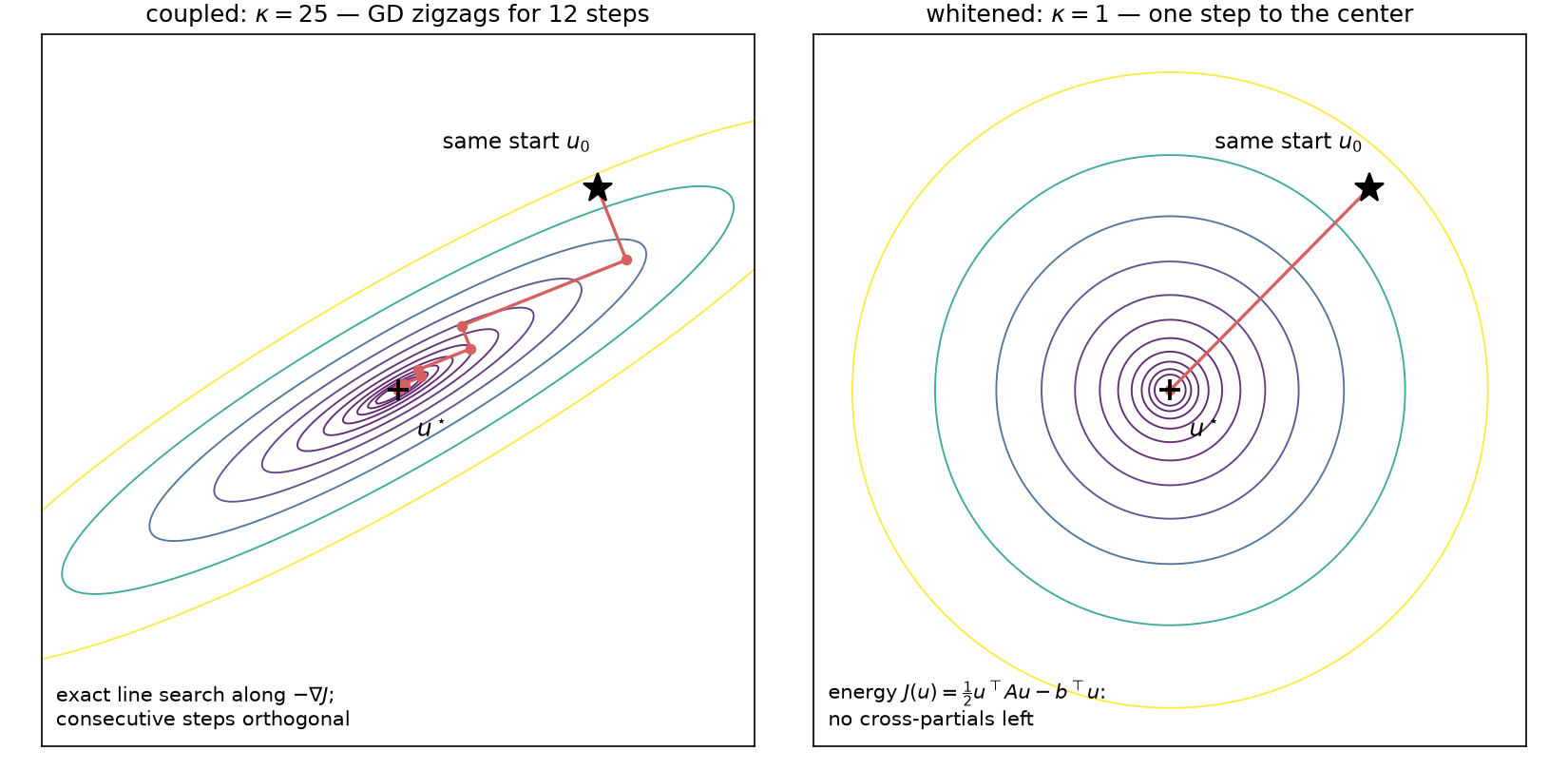
Coupling as landscape: on a coupled quadratic (tilted ellipses, cross-partials nonzero) exact-line-search gradient descent zigzags — 12 steps still leave a $1.04\times10^{-3}$ fraction of the initial error — while in whitened coordinates the contours are circles and the same method lands on the minimizer in exactly one step, the mechanism behind the one-step $7.7\times10^{-17}$ check above.
On the real $A$ the obstruction to this one-liner is the coupling, and “coupling” is not a metaphor for anything — it is the second cross-partial of the energy, measured directly: for five index pairs (grid-E/W neighbors, N/S neighbors, and far pairs), the second-order finite difference $J(u + e_i + e_j) - J(u + e_i) - J(u + e_j) + J(u)$ equals $A_{ij}$ to $4.7\times10^{-10}$ on entries of size $4/h^2 = 4356$ (PASS line 3; the difference is exact for a quadratic — the residue is pure floating-point cancellation). Zero cross-partial $=$ zero precision entry $=$ conditional independence (09 §2): the three vocabularies name one number.
1.2 Why Jacobi does nothing here (the one-paragraph recap of 05/09/12)
Poisson’s diagonal is the constant $4/h^2$, so $\mathrm{diag}(A)^{-1}$ is a scalar — and a scalar decouples nothing, it only rescales the same entangled landscape. Verified as trajectories, not just algebra: Jacobi-GD and plain GD on the rod problem are the same iteration (1998 = 1998 iterations to $10^{-10}$; max relative trajectory deviation over the first 200 iterations $4.7\times10^{-15}$, PASS line 4), the stationary face of 05’s CG no-op (116 = 116) explained statistically in 09 §3 (an independence surrogate with homogeneous conditional variances carries zero correlation information) and priced in 12 §2 ($\rho(B) = \cos(\pi h) = 0.9955$: the perfect two-sided regressions, wasted by a synchronous schedule). Two rate refinements, both verified: on the rod right-hand side GD’s asymptotic $A$-norm rate is $0.988687$, matching $(\kappa_{\mathrm{eff}}-1)/(\kappa_{\mathrm{eff}}+1) = 0.988700$ at the parity-effective $\kappa_{\mathrm{eff}} = 176.00$ — the rod RHS is odd under the 180° rotation (11 §5.2), so the even eigenmodes are exactly unexcited and the lowest live mode is $(1,2)$ at $\lambda = \lambda_1 + \lambda_2 = 49.221$ (PASS lines 5–6); on a generic GRF right-hand side the full-$\kappa$ rate appears: measured $0.995464$ vs $(\kappa-1)/(\kappa+1) = 0.995472 = \cos(\pi h)$, 4753 iterations (PASS lines 7–8). $\kappa$ is a worst-case-RHS bound, and the parity subtlety is logged as a deviation.
1.3 The exact decoupler: rotate to the eigenbasis (= KL/PCA whitening)
There is a basis in which Poisson is §1.1: the 2-D DST-I basis $V_2 = V_1 \otimes V_1$. Verified: $V_2$ is orthonormal ($\max\vert V_2^\top V_2 - I\vert = 1.0\times10^{-14}$), diagonalizes $A$ (max off-diagonal of $V_2^\top A V_2$: $3.3\times10^{-15}$ relative; diagonal $= \lambda_i + \lambda_j$ to $5.3\times10^{-15}$), and the one-pass solve $x = V_2\big((V_2^\top b)/\lambda\big)$ matches spsolve to $1.3\times10^{-15}$ (PASS lines 9–10). In the eigenbasis the problem is 1024 independent scalar parabolas; solving is dividing by the per-mode variance. This is exactly 09 §4.3’s PCA/KL whitening — the eigenbasis is the Karhunen–Loève basis of the field, the frequency-axis representative of the whitener orbit — run as a solver (09 §5’s “spectral solve = KL rotation”, here with the measured receipt). Everything below is about what to do when you cannot afford the exact rotation: pick an axis of decoupling — coordinates, frequency, direction, space, scale — split along it cheaply, and let the iteration absorb what the split misses.
2. Separable: heat diffusion is row-coupling plus column-coupling
2.1 The Kronecker sum, exactly
The requested worked example. The 2-D Laplacian is a Kronecker sum of two 1-D operators,
\[A \;=\; H + V, \qquad H = (I \otimes d_1)/h^2, \qquad V = (d_1 \otimes I)/h^2,\]and on this grid the split is verified exactly, not to machine precision: $\max\vert H + V - A\vert = 0.0$ and — the load-bearing structural fact — $H$ and $V$ commute exactly, $\max\vert HV - VH\vert = 0.0$ (PASS lines 11–12; Kronecker algebra: $HV = VH = (d_1 \otimes d_1)/h^4$). The Wolfram script re-proves both in exact integer arithmetic: max|A - (H+V)| (exact) = 0, max|H.V - V.H| (exact) = 0. Commuting means simultaneously diagonalizable — one shared eigenbasis, the separable $\sin\otimes\sin$ modes — which is why the spectrum is the sum set ${\lambda_i + \lambda_j}$ (verified against the dense eigensolve to $3.1\times10^{-15}$, PASS line 13).
Physically: heat diffusion on the grid is row-coupling plus column-coupling and nothing else. Verified block-anatomy (PASS lines 14–15): reshaped to grid indices, $H$ has exactly zero coupling mass between different grid rows, and all 32 of its diagonal blocks equal $d_1/h^2$ exactly — $H$ alone is 32 independent 1-D heated rods, one per grid row, each of them the chain of 09 — while $V$ couples only within grid columns (cross-column mass exactly 0). Each half, taken by itself, is embarrassingly decoupled: $(H + \sigma I)x = y$ splits into 32 independent tridiagonal solves, one per row (verified against spsolve to $2.9\times10^{-16}$; same for $V$ by columns, PASS line 16), each of them the $O(n)$ Thomas/Kalman pass of 09 §5. The whole difficulty of the 2-D problem is that the two trivially-solvable halves must hold simultaneously.
2.2 The cheap decoupler: one ADI double-sweep as a preconditioner
So build the preconditioner that solves the two halves in sequence — one rows pass, one columns pass:
\[M^{-1} \;=\; 2\sigma\,(V + \sigma I)^{-1}(H + \sigma I)^{-1}, \qquad \sigma = \sqrt{\lambda_1 \lambda_n} = 207.032,\]with $\lambda_1 = 9.8622$, $\lambda_n = 4346.14$ the extreme 1-D eigenvalues. This is one double-sweep of the alternating-direction implicit iteration of Peaceman & Rachford (1955) with a single geometric-mean shift, frozen into an SPD $M$. Cost: one apply = 32 row tridiagonal solves + 32 column tridiagonal solves = 64 tridiagonal solves, $O(N)$ — the same order as one sparse matvec with $A$. Verified: commuting SPD factors make $M^{-1}$ symmetric (asymmetry $4.9\times10^{-16}$) and positive (eigenvalues in $[2.0\times10^{-5}, 8.8\times10^{-3}]$), and the banded-solve apply agrees with the dense $M^{-1}r$ to $5.4\times10^{-16}$ (PASS line 17).
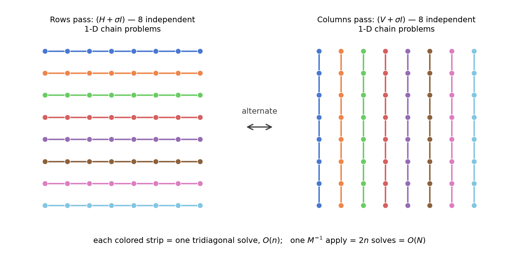
The two problems we are solving: the rows pass $(H + \sigma I)$ is a stack of independent 1-D chains, one per grid row, and the columns pass $(V + \sigma I)$ the same per column (schematic drawn on an $8\times8$ grid for legibility) — which is why one apply of $M^{-1}$ costs 64 tridiagonal solves, $O(N)$, on the real $32\times32$ problem.
Because everything commutes, the preconditioned spectrum has a closed form, verified eigenvalue-by-eigenvalue (max dev $3.4\times10^{-15}$, PASS line 18; Wolfram independently: $8.0\times10^{-15}$ relative on the dense eigensolve):
\[\mathrm{spec}(M^{-1}A) \;=\; \left\{ f(\lambda_i, \lambda_j) = \frac{2\sigma(\lambda_i + \lambda_j)}{(\lambda_i + \sigma)(\lambda_j + \sigma)} \right\}_{i,j=1}^{n}.\]The geometric-mean shift balances the corners (PASS line 19): $f(\lambda_1, \lambda_1) = f(\lambda_n, \lambda_n) = 0.173609$ exactly (rel dev $1.6\times10^{-16}$) — the all-smooth and all-rough modes, treated identically — with the minimum at those pure corners and the maximum $f(\lambda_1, \lambda_n) = 1.826391$ at the mixed corner $(1, 32)$: the surviving difficulty is exactly the modes that are smooth along one axis and rough along the other, the modes on which the rows-expert and the columns-expert disagree most. Two tidy consequences, both pure algebra confirmed by the measured numbers: $f_{\min} + f_{\max} = 0.173609 + 1.826391 = 2$ exactly (the 13-report echo of 12 §2’s $\lambda_{\min} + \lambda_{\max} = 8/h^2$ coincidence — so the undamped Richardson sweep with this $M$ is already optimally damped, $\rho(I - M^{-1}A) = 1 - f_{\min} = 0.826$), and
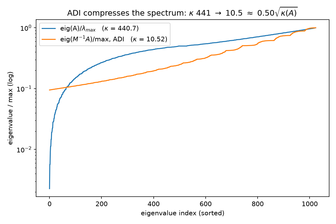
\[\kappa(M^{-1}A) \;=\; \frac{f_{\max}}{f_{\min}} \;=\; \frac{1 + \kappa}{2\sqrt{\kappa}} \;=\; \frac{\sqrt{\kappa}}{2}\Big(1 + \frac{1}{\kappa}\Big).\]The square-root effect, measured: $\kappa(M^{-1}A) = 10.5201 = 0.501\sqrt{\kappa(A)}$ (PASS line 20), against $\sqrt{440.6886}/2 = 10.4963$ — the Wolfram script checks the same two numbers independently and confirms the ratio to within its 2% tolerance (kappa(Minv.A) = 10.520109666, Sqrt[kappa(A)]/2 = 10.496291730); the residual factor is exactly the $1 + 1/\kappa$ above. One ADI double-sweep converts an $O(h^{-2})$ conditioning problem into an $O(h^{-1})$ one:
(Independent Wolfram rendering: 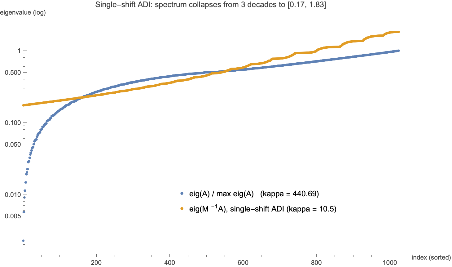 .) Solver receipts (error criterion $\Vert x_k - x^\star\Vert /\Vert x^\star\Vert \le 10^{-10}$, rod problem): ADI-CG 32 iterations, ADI-GD 88 — against 73 and 1998 unpreconditioned (§4’s ladder). Read it as the thesis instructs: the rows pass optimizes the 32 row-subproblems exactly and separately, the columns pass the 32 column-subproblems; the coupling between the passes — the mixed modes — is what remains, and its price is $\kappa’ \approx \tfrac12\sqrt{\kappa}$. (The literature completes the ladder rung: each doubling of a well-chosen cycled-shift ladder square-roots the effective condition number again — $2^{J-1}$ shifts give $\kappa’ = O(\kappa^{1/2^J})$ — so $O(\log\kappa)$ sweeps reach $\kappa’ = O(1)$ on commuting model problems: Wachspress’s ADI model problem; our single-shift $M$ is the $J = 1$ rung, and the only one machine-checked here.)
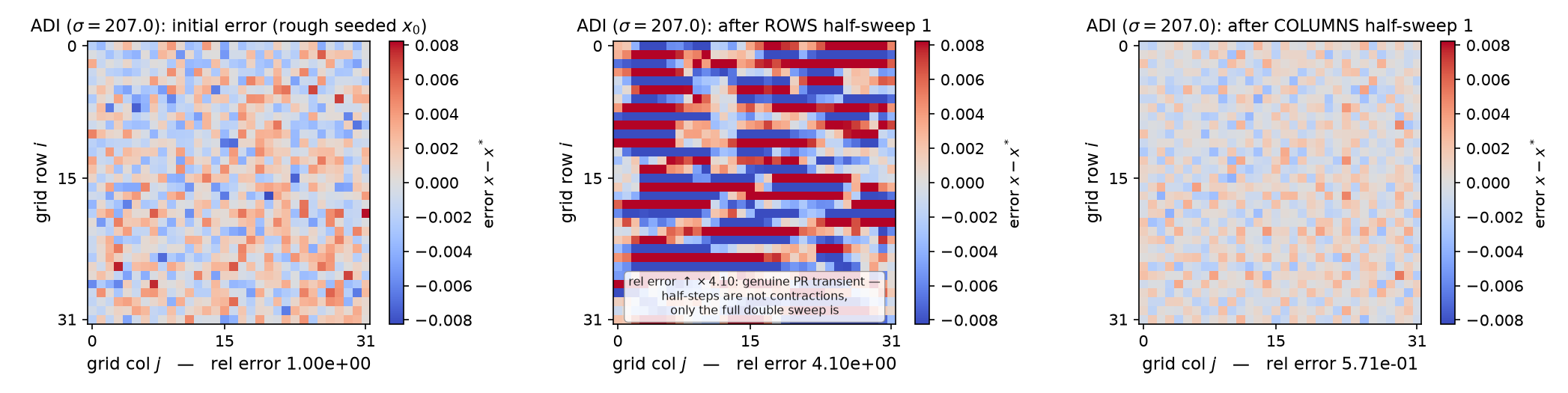
Watch each half-sweep wipe the error along one direction on the real $32\times32$ rod problem ($\sigma = 207.032$): the rows half-sweep leaves bold horizontal stripes, the columns half-sweep erases them (the rel-error readout momentarily rises after a rows half-sweep — $\times 4.10$ on the first one, worst case $5.05\times$ — a genuine Peaceman–Rachford transient: half-steps are not contractions, only the full double sweep is), and the measured per-double-sweep tail rate 0.7885 approaches $(\sigma-\lambda_1)^2/(\sigma+\lambda_1)^2 = 0.8264 = 1 - f_{\min}$, exactly the $\rho(I - M^{-1}A) = 0.826$ quoted above. (Static key frames: anim13_adi_sweep_frames.png; the schematic above is $8\times8$ for legibility, the experiments are $32\times32$.)
Interactive: drag through the sweeps yourself — a slider over ADI half-sweeps on the hot-rod/cold-rod plate.
3. Semiseparable: the solution operator has reduced interactions built in
The previous section decoupled the operator. This one is about a structural fact of the inverse — the object every preconditioner is trying to imitate.
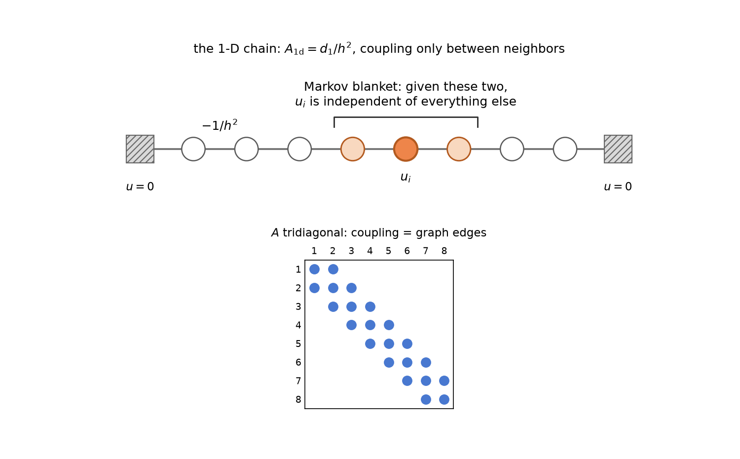
The chain whose inverse this section dissects: each interior node’s energy has cross-partials only with its two spring-coupled neighbors (entries $-1/h^2$ of the tridiagonal $d_1/h^2$), so those two neighbors are the node’s Markov blanket — the 1-D miniature of §4’s two-column separator.
1-D: the inverse of the tridiagonal chain is semiseparable — a rank-1 triangle. Verified (PASS line 21): for $A_{1\mathrm d} = d_1/h^2$,
\[\big(A_{1\mathrm d}^{-1}\big)_{ij} \;=\; h\,x_i\,(1 - x_j) \quad \text{for } i \le j,\]max relative dev $1.4\times10^{-15}$ — and the Wolfram script proves it exactly in rationals (max|Inverse(d1/h^2)_ij - h x_i (1 - x_j)|, i<=j (exact) = 0). This is 09 §2’s Brownian-bridge covariance $h(\min(s,t) - st)$ re-read structurally: the entire upper triangle of the dense inverse is the outer product of two vectors, $u_i = h x_i$ and $v_j = 1 - x_j$ (rank 1!), while the full matrix still has full rank 32. Dense does not mean unstructured: $n^2$ correlations are carried by $O(n)$ numbers. That is Gantmacher–Krein’s classical “one-pair” (Green’s) matrix theorem — the inverse of an irreducible tridiagonal is semiseparable — and it is why the $O(n)$ Thomas/Kalman solve of 09 §5 exists at all.
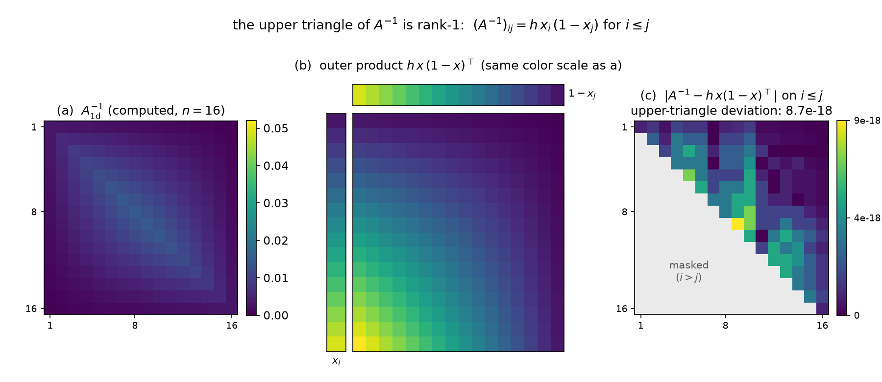
The identity in pixels: the upper triangle of the dense $(d_1/h^2)^{-1}$ (left) coincides with the rank-1 outer product $h\,x_i(1-x_j)$ (middle, same color scale); the figure’s own machine check crashes unless the upper-triangle deviation stays below $10^{-12}$ and measures $8.7\times10^{-18}$ absolute at $n=16$ (right) — the same identity verified above at $n=32$ to $1.4\times10^{-15}$ relative, and exactly in rationals by Wolfram.
2-D: far-field blocks of $\Sigma = A^{-1}$ are numerically low-rank. The exact rank-1 triangle does not survive the grid, but its shadow does (PASS line 22): the off-diagonal block of $A^{-1}$ coupling grid rows 0–7 to grid rows 24–31 (a $256\times256$ block, well-separated groups) has numerical rank 11 at the $10^{-8}$ threshold (leading singular value $1.76\times10^{-3}$; the decay curve is the right panel below) — even though $A^{-1}$ is entrywise dense and strictly positive (min entry $2.9\times10^{-9} > 0$, the M-matrix positivity of 11 §1.1) and full-rank ($\lambda_{\min} = 1.15\times10^{-4} > 0$).
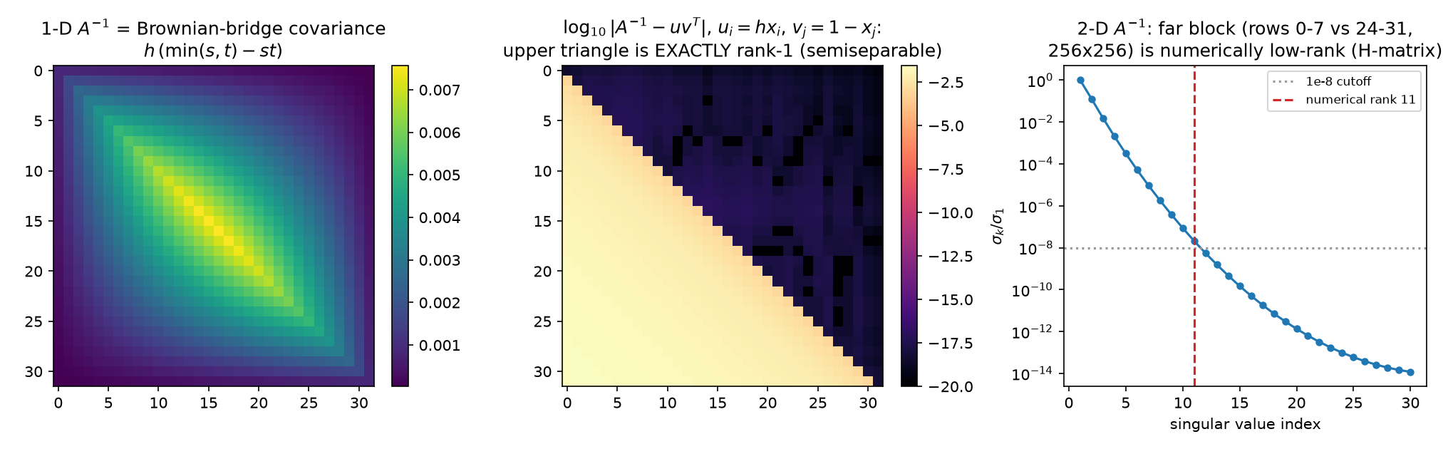
The statistical reading: between two well-separated regions, the $256^2$ pairwise covariances are routed through $\approx 11$ effective degrees of freedom — long-range dependence is low-dimensional, the far field interacts through a few smooth “factors” (the screening effect of 12 §3, seen from the covariance side). The numerical-analysis reading: this is the defining compression of hierarchical ($\mathcal H$-) matrices (Hackbusch): partition $A^{-1}$ by an admissibility condition and store far blocks as low-rank factors, giving $O(N\log N)$ approximate inverses — with the guarantee that elliptic inverses admit exactly this structure (Bebendorf–Hackbusch). The moral for the thesis: reduced interactions are not only something you impose on the problem; the solution operator already has them. Decoupling schemes work because the object they approximate is itself nearly decoupled at long range. (14 follows this section to its algorithmic conclusion: the separator theorem behind these ranks, the full HODLR anatomy of $A^{-1}$, and the compressed inverse run as a preconditioner.)
4. Space: two subdomains, one interface, and the decoupling ladder
4.1 Conditional independence across a separator is exact (the statistics name for decoupling)
Split the grid by the two middle columns: $L$ = columns 0–14, $I$ = columns 15–16, $R$ = columns 17–31. The 5-point stencil puts no precision edge across the separator: $\mathrm{nnz}(A_{LR}) = 0$ (PASS line 23). The GMRF global Markov property (Rue & Held) then promises exact conditional decoupling, and the experiment collects it from the dense covariance (PASS line 24):
\[\mathrm{Cov}(u_L, u_R \mid u_I) \;=\; \Sigma_{LR} - \Sigma_{LI}\Sigma_{II}^{-1}\Sigma_{IR} \;=\; 0 \quad\text{exactly: } \max\vert \cdot\vert = 1.9\times10^{-19},\]against a marginal $\max\vert \Sigma_{LR}\vert = 2.6\times10^{-4}$ — a ratio of $7.2\times10^{-16}$, i.e. fifteen orders of magnitude of dependence annihilated by conditioning on 64 interface values. Marginally the halves are thoroughly coupled (§3’s dense positive $\Sigma$); given the interface they are independent. This is the same statement as §2’s, on a different axis: there the two sub-physics shared an eigenbasis; here they share only a 2-column Markov blanket.
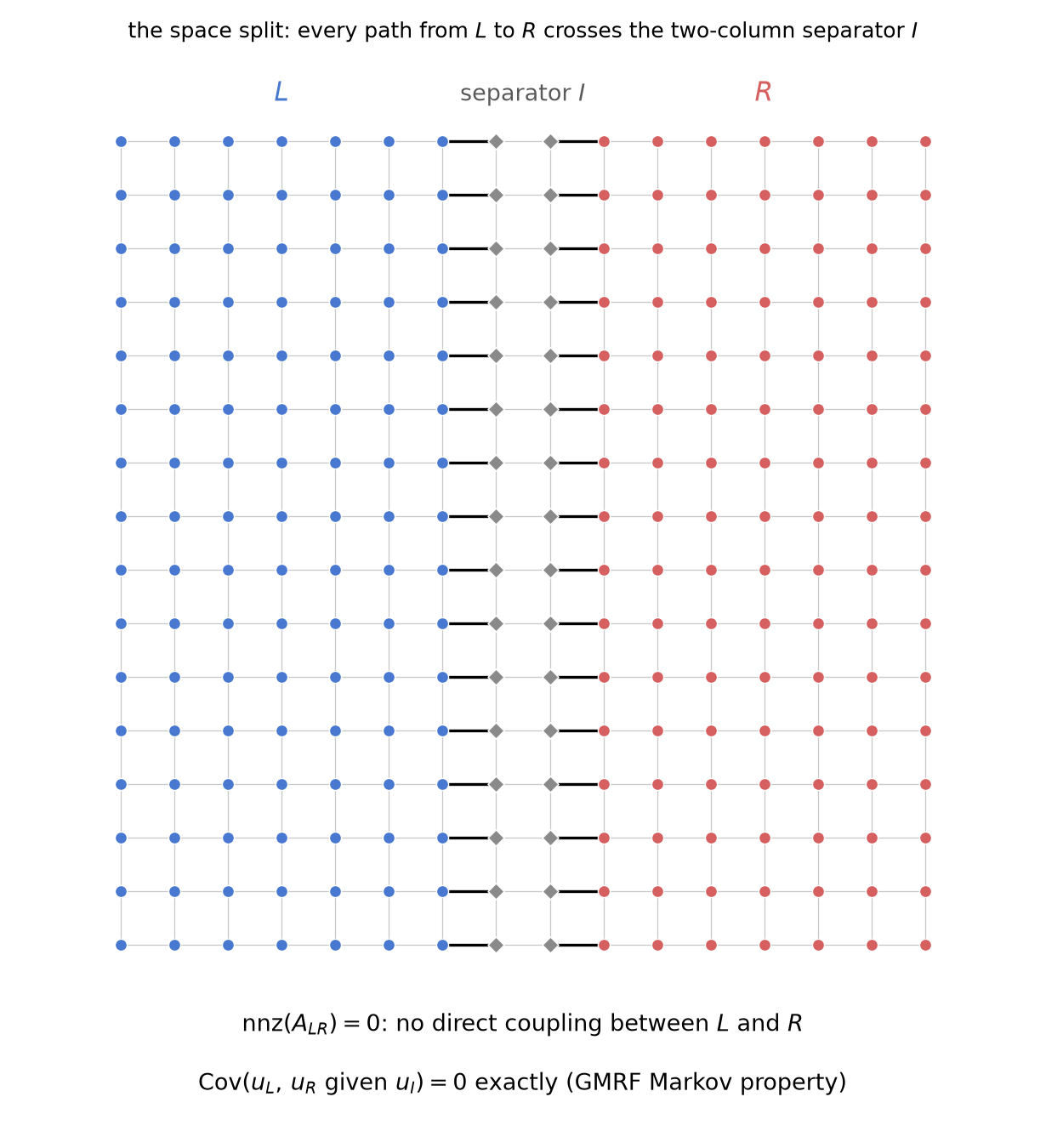
The split drawn on the stencil graph (a $16\times16$ grid for legibility): every 5-point edge from $L$ to $R$ passes through the shaded separator columns, and the figure machine-checks $\mathrm{nnz}(A_{LR}) = 0$ on poisson_2d(16) before drawing — the same exact zero verified above at $n = 32$ (PASS line 23).
4.2 Block-Jacobi(2): optimize each half with the other frozen
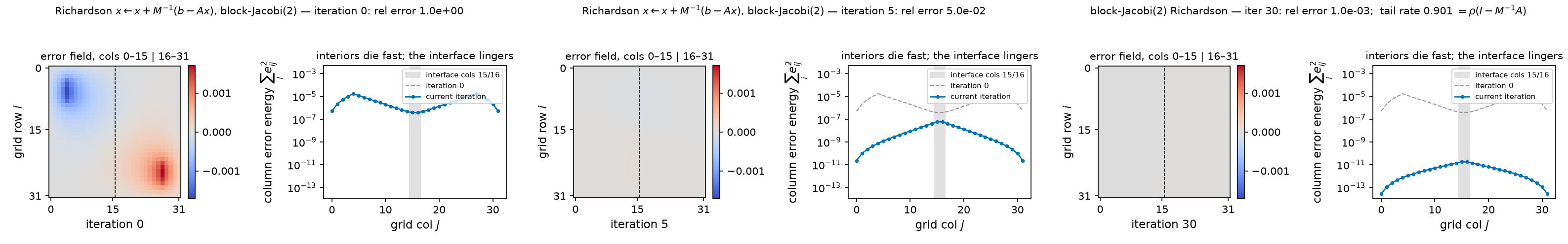
The preconditioner this licenses: split into halves $L’$ = columns 0–15, $R’$ = columns 16–31 and take $M = \mathrm{blockdiag}(A_{L’L’}, A_{R’R’})$ — one exact $32\times16$ Poisson solve per subdomain, “optimize each half pretending the other is frozen” (the additive-Schwarz / nonoverlapping domain-decomposition move; Schwarz 1870, Smith–Bjørstad–Gropp, Toselli–Widlund). What remains is provably only the interface, and it is low-dimensional and localized (PASS lines 25–26):
- $A_{L’R’}$ has exactly 32 nonzeros — one column of edges — and rank 32. Since $A - M$ is this rank-64 (two-sided) perturbation, $M^{-1}A$ has eigenvalue 1 with multiplicity $960 = N - 2\cdot32$: on a 960-dimensional subspace the frozen-half model is already exact. The remaining 64 eigenvalues split symmetrically in pairs $1 \pm \mu$ (pairing deviation $4.4\times10^{-15}$), 32 distinct $\mu$’s running up to $\mu_{\max} = 0.9014$: $\mathrm{spec}(M^{-1}A) \subset [0.0986, 1.9014]$ with $\lambda_{\min} = 1 - \mu_{\max} = 0.0986$, $\kappa(M^{-1}A) = 19.29$. (Again $\lambda_{\min} + \lambda_{\max} = 2$: the undamped Richardson sweep is optimally damped, $\rho(I - M^{-1}A) = 0.9014$ — one frozen-halves sweep leaves 90% of the worst mode, 12 §1’s currency.)
- The extreme eigenvectors of the preconditioned operator localize at the interface: the $\lambda_{\min} = 0.0986$ eigenvector’s column-energy profile peaks at column 16 and the $\lambda_{\max} = 1.9014$ one at column 15, with columns 14–17 carrying 39% of the $\lambda_{\min}$ mode’s energy:
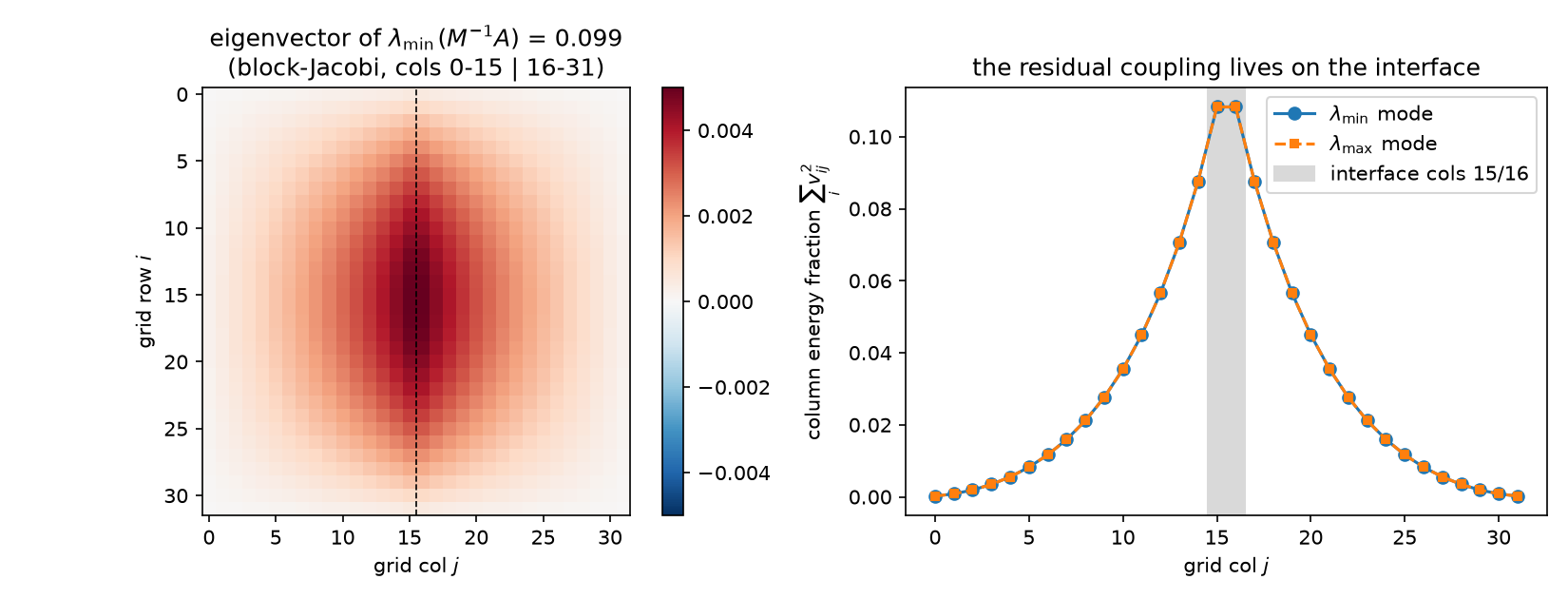
Solver receipts: blockJacobi2-CG 12 iterations (GD: 98). Twelve is far below the $\sqrt{\kappa’}$ heuristic and even below ADI’s 32 at smaller $\kappa’$ — because the spectrum is 960 exact 1’s plus 64 stragglers, at most 65 distinct eigenvalues, and CG’s currency is clusters (§5.3). The eliminated-interior view is the Schur complement: solving the halves exactly reduces the global problem to an effective equation on the interface (the Dirichlet-to-Neumann operator, 12 §3’s decimation row) — a rank-32 problem, which is what those 64 non-unit eigenvalues are the spectrum of. Domain decomposition is the industrialization of exactly this move; and the reason practical DD adds a coarse space is 11 §5’s reason: the interface modes that survive are smooth along the interface, i.e. the residual coupling is not only low-rank but low-frequency — the space axis hands off to the scale axis.
The frozen-halves iteration in motion (rod problem): the subdomain interiors die within a few sweeps while the interface mode lingers — columns 14–17 still carry 42% of the error energy at iteration 30 — and continuing the same iteration to 200 sweeps measures a tail rate of 0.901444, matching the $\rho(I - M^{-1}A) = 0.9014$ above to six digits. (Static key frames: anim13_interface_frames.png.)
4.3 The decoupling ladder
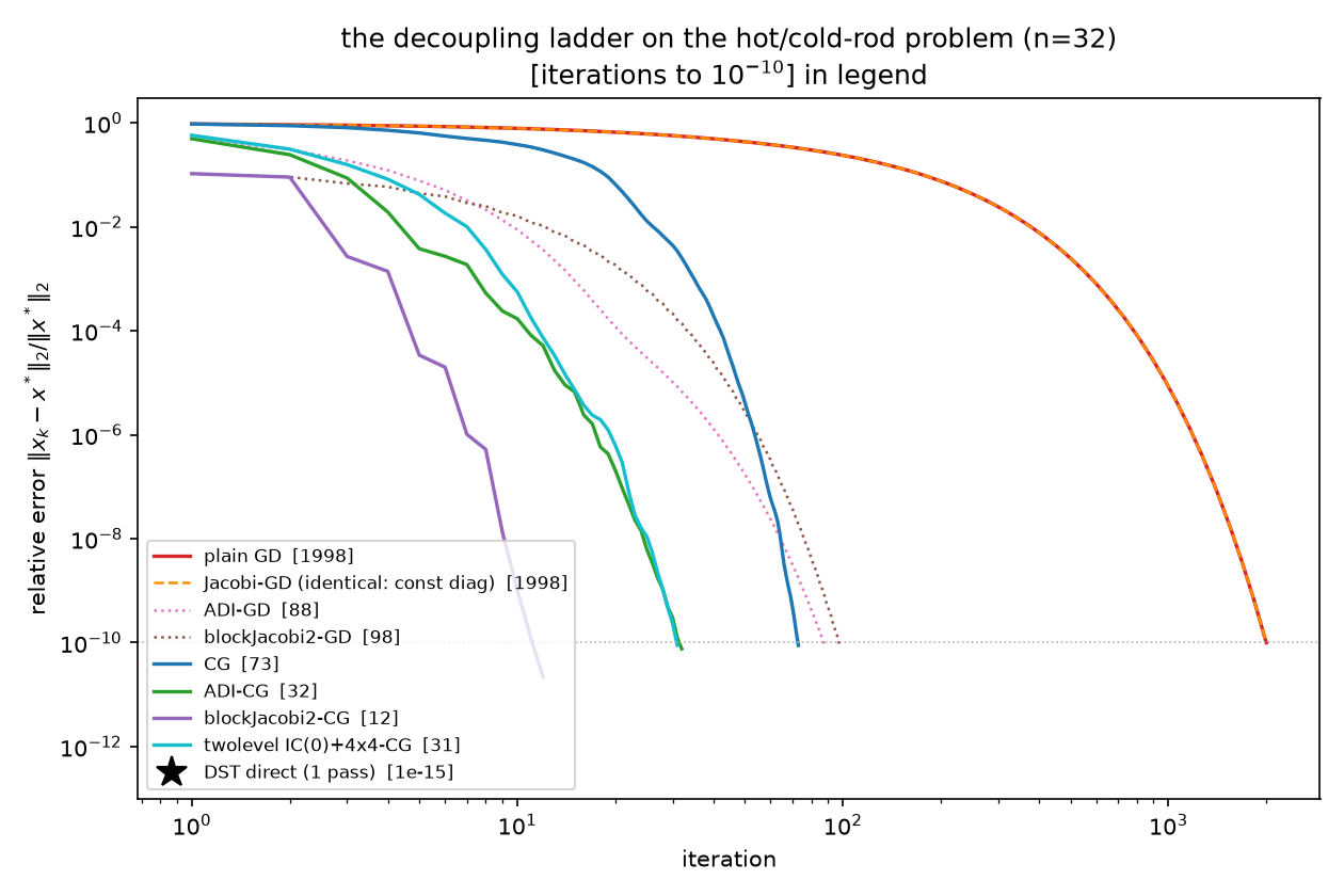
One move — pick an axis, split exactly along it, approximate the rest — five axes. All numbers measured on the canonical problem (rod RHS, error criterion $10^{-10}$; $\rho$ = spectral radius of the optimally-damped Richardson sweep, computed from the measured spectral extremes; Jacobi’s from 12 §2):
| axis | exact decoupling condition | verified here as | cheap approximation | $\kappa(M^{-1}A)$ | $\rho(I - M^{-1}A)$ | CG its |
|---|---|---|---|---|---|---|
| coordinates | $A$ diagonal (all coordinates conditionally independent) | diagonal system one-steps ($7.7\times10^{-17}$) | Jacobi $\mathrm{diag}(A)^{-1}$ | 440.69 (unchanged) | 0.9955 | 73 (inert) |
| frequency | known eigenbasis: DST-I diagonalizes $A$ ($3.3\times10^{-15}$) | one-pass KL solve ($1.3\times10^{-15}$) | — (exact; FFT-able) | 1 | 0 | 1 pass |
| direction | $A = H + V$, $[H, V] = 0$ (both exact) | closed-form ADI spectrum ($3.4\times10^{-15}$) | ADI double-sweep, 64 tridiag solves | 10.52 $= 0.50\sqrt{\kappa}$ | 0.826 | 32 |
| space | $\mathrm{Cov}(L, R \mid I) = 0$ (ratio $7.2\times10^{-16}$) | rank-32 interface, 960 unit eigenvalues | block-Jacobi(2), frozen halves | 19.29 | 0.901 | 12 |
| scale | coarse field ⊥ fine residual (approx.; 11 §5.1) | 11/12’s two-level | IC(0) + 4×4 coarse (additive) | 11.05 | 0.834 | 31 |
(PASS line 28 records all the ladder counts and asserts the chains GD > CG > ADI-CG $\ge$ twolevel-CG > 1 and CG > blockJacobi2-CG — the five axes do not order linearly, blockJacobi2’s 12 undercutting twolevel’s 31; the two-level row is 11 §5.2’s best fixed-$M$ method rebuilt verbatim, 31 error-based / 32 residual-based iterations, consistent with 11’s table. Scale’s “exact condition” is the one axis with no finite exact version — hence multigrid recurses it, 05 §5.) The whole ladder on one plot, GD and CG variants together, with the DST one-pass star at the bottom left:
5. GD vs CG: pre-decoupling vs decoupling on the fly
The suite’s remaining question (04 proved the polynomial bounds; here is the decoupling reading, fully measured).
5.1 GD is memoryless: it pays the full eigenvalue range, forever
Steepest descent keeps no state but $x_k$: each step re-solves a 1-D problem along the current gradient and forgets the direction it just optimized. Its asymptotic contraction is set by the range of the spectrum, $(\kappa-1)/(\kappa+1)$ — verified three independent ways in this report: on Poisson ($0.995464$ measured vs $0.995472$, §1.2), and on the rank-1 family below, where the worst-case-RHS rates match $(\kappa-1)/(\kappa+1)$ to seven digits at $\kappa = 101$ ($0.98039214$ measured vs $0.98039216$, rel. dev $1.4\times10^{-8}$) and to all eight printed digits at $10^4{+}1$ and $10^6{+}1$ ($0.99980004$, $0.99999800$; PASS lines 30/33/36). The one thing diagonal preconditioning buys GD — one-stepping — it buys only on the already decoupled problem (§1.1 vs §1.2: $7.7\times10^{-17}$ in one step there, 1998 identical iterations here). A refinement the experiment forced (deviations log): for a generic RHS on a two-eigenvalue problem the textbook rate is provably not attained — the per-step $A$-norm contraction is the exact closed form $\sqrt{f(m_0)}$, $f(m) = (\kappa-1)^2 m /((1+\kappa^2 m)(1+m))$ with $m$ the $\kappa$-weighted mixing ratio of the error components ($m \mapsto 1/(\kappa^2 m)$ is an involution of the GD map and $f$ is invariant under it), verified to the printed digits at all three $\kappa$’s (PASS lines 31/34/37: e.g. measured $0.19548504$ vs predicted $0.19548494$ at $\rho = 10^2$). The worst case is realized exactly by $b = v + w_\perp$ ($m_0 = 1/\kappa$), and that RHS is what the headline numbers below use.
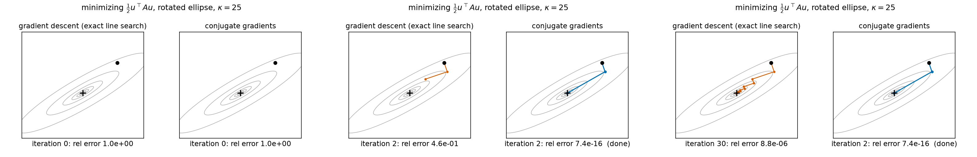
The contrast in one cross-section ($\kappa = 25$, axes rotated 30°, equal-energy error mix $m_0 = 1$): GD zigzags at the constant measured per-step rate 0.6783 — exactly $\sqrt{f(m_0)}$ from the closed form above — reaching only $8.76\times10^{-6}$ after 30 steps, while CG finishes in exactly 2 steps ($7.4\times10^{-16}$), one per distinct eigenvalue. (Static key frames: anim13_gd_vs_cg_frames.png.)
5.2 One global factor is fatal for GD and free for CG
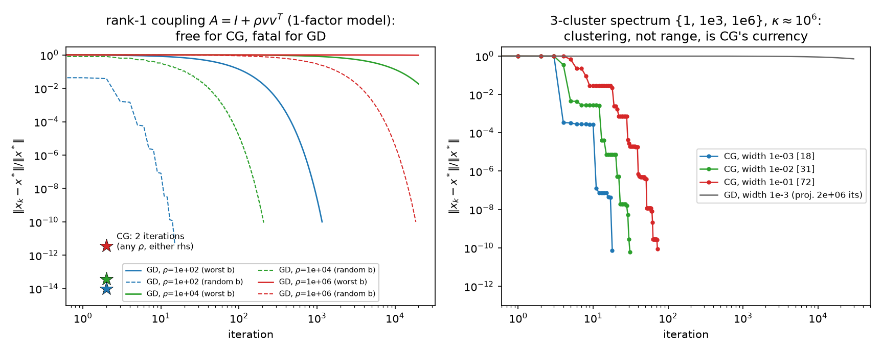
Couple 400 coordinates through a single common factor — the rank-1 perturbation $A = I + \rho\,vv^\top$, a 1-factor covariance model (07’s favorable case, 09 §6’s factor analysis), with coupling strength $\rho = 10^2, 10^4, 10^6$. The spectrum is two points, ${1, 1+\rho}$; $\kappa = 1 + \rho$ is arbitrarily bad while the problem is only one direction away from the identity. Measured (PASS lines 29/32/35/38, figure left panel):
| $\rho$ | $\kappa$ | CG its (rel err after 2, worst-case RHS) | GD its to $10^{-10}$ (worst-case RHS) | $\tfrac{\kappa}{2}\ln 10^{10}$ |
|---|---|---|---|---|
| $10^2$ | $101$ | 2 ($1.3\times10^{-15}$) | 1163 | 1162.8 |
| $10^4$ | $10^4{+}1$ | 2 ($3.7\times10^{-14}$) | 115 141 | 115 140.8 |
| $10^6$ | $10^6{+}1$ | 2 ($3.6\times10^{-12}$) | 11 512 937* | 11 512 937.0 |
CG converges in exactly 2 iterations at every strength, for both random and worst-case RHS (two distinct eigenvalues ⟹ a degree-2 polynomial annihilates the error: the finite-termination clause of CG’s minimax optimality, 04, Hestenes–Stiefel). GD’s count grows linearly in $\kappa$ — the measured counts match $\tfrac{\kappa}{2}\ln(10^{10})$ to $\le 0.02\%$ (last column — the asymptotic of the exact $\ln(10^{10})/{-\ln\tfrac{\kappa-1}{\kappa+1}}$, which itself rounds to precisely the measured counts). *The $\rho = 10^6$ run hit the 120 000-iteration cap at relative error 0.79 and is extrapolated from the measured (provably constant) per-step rate — deviations log, entry 1.
5.3 Clusters, not range: the 3-cluster spectrum
Now three clusters — eigenvalue centers ${1, 10^3, 10^6}$ with multiplicities ${300, 80, 20}$ and relative widths $w$, so $\kappa \approx 10^6$ throughout (PASS lines 39–40, figure right panel):
| cluster width $w$ | $\kappa$ | CG its to $10^{-10}$ | GD |
|---|---|---|---|
| $10^{-3}$ | $1.001\times10^6$ | 18 | rel err 0.72 after 30 000 its; projected $2.1\times10^6$ its |
| $10^{-2}$ | $1.009\times10^6$ | 31 | — |
| $10^{-1}$ | $1.096\times10^6$ | 72 | — |
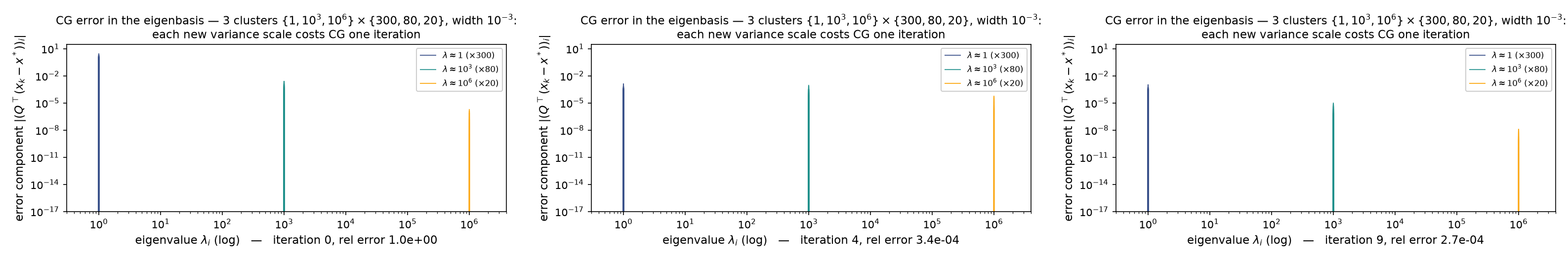
At zero width this would be 3 iterations (three distinct eigenvalues); at width $10^{-3}$ it is 18, degrading only gently as the clusters smear ($18 \to 31 \to 72$) while $\kappa$ sits at $10^6$ the whole time (honesty note: the “$\approx 3$” idealization vs measured 18 is deviations-log entry 5 — CG’s first three sweeps barely move the $\ell_2$ error, 0.996 after 3 iterations, then the largest single sweep drops it 2935× once the Ritz values have found all three clusters). GD, whose only input is the range, is hopeless at any width: measured tail rate 0.9999890 against the worst-case 0.9999980. CG’s currency is the number of (clusters of) distinct eigenvalues; GD’s is the range.
One new variance scale = one CG iteration ($w = 10^{-3}$): the per-cluster eigencomponent bars die cluster by cluster, and the largest single sweep is the 2935× plunge at iteration 4 ($0.99557 \to 3.39\times10^{-4}$) quoted above, once the Ritz values have found all three clusters. (Static key frames: anim13_cg_clusters_frames.png.)
5.4 Why: CG is an on-the-fly sequential decoupler
The mechanism is 09 §5’s row of the dictionary, now with the receipt. CG’s directions satisfy $p_i^\top A p_j = 0$ — measured: max $\vert p_i^\top A p_j\vert /(\Vert p_i\Vert _A\Vert p_j\Vert _A) = 7.3\times10^{-16}$ over the first 10 directions, $1.8\times10^{-15}$ over the first 30 (finite-precision loss growing with depth; PASS line 44). $A$-orthogonality is exactly what “decoupled” means in this report: in the coordinates ${p_i}$, the energy has no cross-partials — $J(x_0 + \sum_i \alpha_i p_i)$ separates into independent scalar parabolas in the $\alpha_i$, so each 1-D minimization is final and never needs revisiting. CG is Gram–Schmidt in the $A$-inner product, run incrementally on the Krylov vectors: statistically, sequential regression on directions that are uncorrelated under the field’s own precision (09 §5: $\mathrm{Cov}(p_i^\top Au, p_j^\top Au) = p_i^\top A p_j$), i.e. the same sequential-whitening move as Cholesky (09 §4.2) but built adaptively from the residuals it encounters. GD, memoryless, keeps re-optimizing directions it has already visited (the classical zigzag); CG never does. That is why the number of distinct variance scales — not their spread — is what CG pays for: each new cluster is one new scalar problem to whiten.
5.5 Pre-decoupling and on-the-fly decoupling compose
Both mechanisms at once, on the ladder (PASS lines 42–43; Chebyshev bound $k \ge \sqrt{\kappa’}\,\ln(2/\varepsilon)/2$ at $\varepsilon = 10^{-10}$, $A$-norm iteration counts; residual-based counts kept comparable to 08’s 116-iteration GRF anchor, re-verified here, PASS line 41):
| $M$ | $\kappa(M^{-1}A)$ | $\sqrt{\kappa’}$ | its ($A$-norm) | Chebyshev bound | bound used | eigenvalues at 1 |
|---|---|---|---|---|---|---|
| none | 440.69 | 20.99 | 75 | 249 | 30% | 0 |
| ADI | 10.52 | 3.24 | 34 | 38 | 88% | 0 |
| blockJacobi(2) | 19.29 | 4.39 | 12 | 52 | 23% | 960 |
| two-level IC(0)+coarse | 11.05 | 3.32 | 32 | 39 | 81% | 9 |
$\sqrt{\kappa’}$ bounds every method (all four counts under their Chebyshev ceilings) — but it does not rank them: the fitted $c = \mathrm{its}/\sqrt{\kappa’}$ spans $[2.96, 11.10]$ and the orderings disagree (ordering_match = False in the JSON). The instructive pair: ADI’s spectrum is a smooth arch with zero eigenvalues at 1 — it burns 88% of its Chebyshev budget, the near-worst-case shape — while blockJacobi(2), with 1.8× larger $\kappa’$, needs a third of ADI’s iterations because 960 of its 1024 eigenvalues sit exactly at 1 and CG only has to learn the 64 stragglers. Spectral shape decides within the bound (deviations-log entry 7 records that this section was reframed after measurement — the data rejected “iterations $= c\sqrt{\kappa’}$” as a fine-grained law). This is the suite’s oldest scar, finally explained end-to-end: 06’s NPO wins 3.87× entirely by clustering, and 07’s Nyström fails despite attacking $\kappa$, because Krylov methods buy convergence with clusters, and $\kappa$ is merely the crudest summary of clustering. Punchline: a preconditioner decouples ahead of time; CG decouples as it goes; and they compose — the preconditioner collapses the spectrum toward few effective scales, CG whitens whatever scales are left, one per (cluster of) eigenvalue.
6. Dictionary delta
Rows appended to 09 §8, 11 §7, 12 §6 — all machine-checked in decoupling.py / decoupling_adi.wls except the row marked †, which is the standard structural analogy:
| Numerical linear algebra / PDE | Statistics / probability |
|---|---|
| Cross-partial $\partial^2 J/\partial u_i\partial u_j = A_{ij}$ (FD-verified, $4.7\times10^{-10}$ on entries of size 4356) | Conditional dependence of $u_i, u_j$ given the rest; off-diagonal precision |
| Diagonal $A$: $N$ independent parabolas, GD one-steps ($7.7\times10^{-17}$) | Fully independent coordinates; inference = $N$ scalar problems |
| Separable (Kronecker-sum) operator $A = H + V$, $[H,V] = 0$ exactly | Two commuting sub-physics = two independent Gaussian information sources about one field; precision adds, one shared KL basis diagonalizes both |
| ADI double-sweep $2\sigma(V{+}\sigma I)^{-1}(H{+}\sigma I)^{-1}$ | Alternating conditional optimization — coordinate descent by direction (rows pass, then columns pass), backfitting the two sub-models |
| Geometric-mean shift $\sigma = \sqrt{\lambda_1\lambda_n}$; $f_{\min}{+}f_{\max} = 2$ | Equalizing the two experts’ worst mismatch; hardest surviving modes = where the experts disagree (mixed corner $(1, 32)$) |
| Semiseparable inverse: $h\,x_i(1-x_j)$ rank-1 triangle (exact); far blocks of $\Sigma$ rank-11/256 | Long-range dependence carried by few effective factors; screening from the covariance side; $\mathcal H$-matrix admissibility† |
| Separator (columns 15–16); $\mathrm{nnz}(A_{LR}) = 0$ | Markov blanket: $\mathrm{Cov}(L, R \mid I) = 0$ exactly ($7.2\times10^{-16}$) |
| Block-Jacobi(2): frozen-halves solves; eigenvalue 1, multiplicity $960 = N - 2\,\mathrm{rank}(A_{LR})$ | Optimize each half with the other clamped; directions the surrogate already whitens exactly |
| Schur complement / interface problem; extreme modes localized at columns 15/16 | Effective interface physics after marginalizing the interiors; residual coupling is low-dimensional (rank 32) and lives on the blanket |
| CG conjugacy $p_i^\top A p_j = 0$ ($1.8\times10^{-15}$ over 30 directions) | Sequential decorrelation: on-the-fly Gram–Schmidt in the precision metric = adaptive sequential regression (09 §5) |
| Two distinct eigenvalues ⟹ CG = 2 its (measured at $\kappa$ up to $10^6$) | One common factor + noise: two variance scales = two regressions, however strong the factor |
| GD rate $(\kappa-1)/(\kappa+1)$ (measured to 7–8 digits); its $\approx \tfrac{\kappa}{2}\ln\tfrac1\varepsilon$ | Memoryless learner: pays the full variance range every step, relearns old directions; refinement $\sqrt{f(m_0)}$ for generic data |
| $\kappa$ bound vs clustering (88% vs 23% Chebyshev utilization) | Worst-case spread vs number of distinct variance scales actually present |
7. Pointers
ADI is Peaceman & Rachford (J. SIAM 3, 1955) and Douglas & Rachford (1956); the shift theory and the $O(\log\kappa)$ multi-shift result are Wachspress (The ADI Model Problem, 1995; also Varga, Matrix Iterative Analysis, ch. 7). Semiseparability of tridiagonal inverses is Gantmacher & Krein (Oscillation Matrices and Kernels, 1941/2002); the modern treatment is Vandebril, Van Barel & Mastronardi (Matrix Computations and Semiseparable Matrices, 2008); hierarchical matrices are Hackbusch (Computing 62, 1999; Hierarchical Matrices, 2015), with the elliptic-inverse approximability theorem in Bebendorf & Hackbusch (Numer. Math. 95, 2003). The GMRF Markov property and separator calculus are Rue & Held (Gaussian Markov Random Fields, 2005) — the same source as 09’s half of the dictionary. Domain decomposition: Schwarz (1870), the modern theory in Smith, Bjørstad & Gropp (1996) and Toselli & Widlund (Domain Decomposition Methods, 2005) — including why two-level (coarse-space) corrections are mandatory, which is 11 §5’s measurement wearing DD clothes. CG’s minimax optimality and finite termination are Hestenes & Stiefel (1952) via 04; the clustering refinements are Axelsson & Lindskog (1986) and van der Sluis & van der Vorst (1986); Greenbaum (Iterative Methods for Solving Linear Systems, 1997) for both. The GD zigzag asymptotics go back to Akaike (1959). Siblings: the operator and spectrum, 01/02; the GRF RHS, 03; the baselines, 05; the clustering win and the $\kappa$-reduction failure, 06/07; consolidated tables, 08; the dictionary, physics, grid, and Richardson readings, 09/10/11/12; the roadmap, 00.
Coda. Reports 05–13 are one statement. The energy $J$ has cross-partials; the cross-partials are the precision’s off-diagonal; the off-diagonal is conditional dependence — and every solver move in the suite is a decision about which of those interactions to model exactly, which to approximate, and which to leave for the iteration to discover. Model none of them: Jacobi, and the iteration discovers everything at $\cos(\pi h)$ per sweep. Model them all: the DST rotation or the perfect autoregression, one pass, nothing left to discover. In between, choose an axis and split: rows from columns (ADI, exactly separable, $\kappa \to \tfrac12\sqrt\kappa$), left from right (block-Jacobi, halves exactly conditionally independent given the 64 interface values of §4.1’s two-column separator, all residual coupling localized there), coarse from fine (11/12’s two-level, the one axis that must be recursed). What the split leaves unmodeled is a number — $\rho(I - M^{-1}A)$ per sweep, or $\kappa(M^{-1}A)$ with its clusters for CG — and CG itself is the same move made adaptive: a sequential decoupler that whitens one surviving scale per iteration and therefore counts clusters where gradient descent counts the whole range. Solving a coupled system is uncoupling it; the only choices are the axis, the price, and whether you pay before the iteration or during it.