02 — The Eigenvalue Story of $d_1$ and $A$
This report derives, from scratch, the complete spectral theory of the two matrices this repo is built on:
- $d_1$ — the $n \times n$ one-dimensional Dirichlet second-difference stencil (tridiagonal $[-1, 2, -1]$), built in python/poisson.py lines 35–40;
- $A = (d_1 \otimes I + I \otimes d_1)/h^2$ — the $n^2 \times n^2$ five-point 2-D discrete Laplacian, built in python/poisson.py lines 64–68, with $h = 1/(n+1)$.
Everything is closed-form. Every formula below is verified numerically in python/experiments/spectra.py (output: results/spectra.json) and independently in Mathematica by mathematica/eigen_check.wls. The headline numbers at $n = 32$ ($N = n^2 = 1024$):
| quantity | analytic | computed (eigvalsh) |
max deviation |
|---|---|---|---|
| $\mathrm{spec}(d_1)$ | $2 - 2\cos\frac{k\pi}{n+1}$ | dense eigensolve | $2.22 \times 10^{-15}$ |
| $\mathrm{spec}(A)$ | $(\lambda_k + \lambda_l)/h^2$ | dense eigensolve | $2.73 \times 10^{-11}$ |
| $\lambda_{\min}(A)$ | $19.72430527164353$ | $19.724305271649925$ | — |
| $\lambda_{\max}(A)$ | $8692.275694728356$ | $8692.27569472836$ | — |
| $\kappa(A)$ | $440.6885603836582$ | $440.6885603835139$ | $3.3\times10^{-13}$ relative |
(All values from results/spectra.json.) The $2.73\times10^{-11}$ absolute deviation for $A$ is not worse conditioning of the eigensolve — it is machine epsilon at the scale of the eigenvalues: $2.73\times10^{-11}/8692 \approx 3\times10^{-15}$, i.e. the same $\sim$ few-ulp relative accuracy as the 1-D check.
Cross-links: the matrices themselves are walked through in 01-code-walkthrough.md; the right-hand side these matrices are solved against is 03-gaussian-random-fields.md; the consequence of this spectrum for CG iteration counts is 04-krylov-and-pcg.md; what preconditioners do to this spectrum is §8 below and 05-classical-preconditioners.md, 06-neural-preconditioner.md, 07-nystrom-preconditioning.md; the full experimental table is 08-results.md.
1. Setup: the eigenproblem for $d_1$
$d_1$ discretizes $-u’’$ on $(0,1)$ with homogeneous Dirichlet data $u(0) = u(1) = 0$, on the $n$ interior nodes $x_j = jh$, $j = 1, \dots, n$, $h = 1/(n+1)$ (the stencil matrix carries no $1/h^2$ factor — that is applied once, in 2-D, at python/poisson.py:67). Row $j$ of the eigenproblem $d_1 v = \lambda v$ reads
\[-v_{j-1} + 2v_j - v_{j+1} = \lambda v_j, \qquad j = 1, \dots, n,\]where the boundary conditions enter as the convention
\[v_0 = 0, \qquad v_{n+1} = 0.\]This is exactly a linear three-term recurrence in $j$ with two boundary constraints — a discrete two-point boundary value problem. We solve it the way one solves any constant-coefficient linear recurrence.
2. Derivation of the sine eigenvectors from the recurrence
Step 1 — characteristic equation. Rewrite the recurrence as
\[v_{j+1} - (2 - \lambda)\, v_j + v_{j-1} = 0 .\]Seek solutions $v_j = r^j$. Substituting gives the characteristic polynomial
\[r^2 - (2 - \lambda)\, r + 1 = 0 ,\]with roots $r_\pm$ satisfying
\[r_+ r_- = 1, \qquad r_+ + r_- = 2 - \lambda .\]The roots are reciprocal. Write $r_+ = r$, $r_- = r^{-1}$; the general solution (for $r \neq \pm 1$, i.e. distinct roots) is
\[v_j = \alpha\, r^j + \beta\, r^{-j}.\]Step 2 — impose the left boundary. $v_0 = \alpha + \beta = 0$ forces $\beta = -\alpha$, so
\[v_j = \alpha\left(r^j - r^{-j}\right).\]Step 3 — impose the right boundary. $v_{n+1} = \alpha\left(r^{n+1} - r^{-(n+1)}\right) = 0$ with $\alpha \neq 0$ (else $v \equiv 0$) requires
\[r^{2(n+1)} = 1 ,\]so $r$ is a $2(n+1)$-th root of unity:
\[r = e^{i\theta_k}, \qquad \theta_k = \frac{k\pi}{n+1}, \qquad k \in \mathbb{Z}.\]Since $d_1$ is symmetric its eigenvalues are real, and indeed $\vert r\vert = 1$ makes $\lambda = 2 - (r + r^{-1}) = 2 - 2\cos\theta_k$ real automatically. The values $k = 1, \dots, n$ give distinct $\theta_k \in (0, \pi)$ hence distinct eigenvalues ($2 - 2\cos\theta$ is strictly increasing on $(0,\pi)$); $k = 0$ and $k = n+1$ give $r = \pm 1$ (the excluded repeated-root cases) and only the trivial solution; $k > n+1$ and $k < 0$ repeat the same eigenvectors up to sign. So we have exactly $n$ eigenpairs — the complete spectrum.
Step 4 — read off the eigenvector. With $r = e^{i\theta_k}$,
\[v_j = \alpha\left(e^{ij\theta_k} - e^{-ij\theta_k}\right) = 2i\alpha \sin(j\theta_k),\]so choosing $\alpha = 1/(2i)$:
\[\boxed{\; v^{(k)}_j = \sin\!\left(\frac{jk\pi}{n+1}\right) = \sin(k\pi x_j), \qquad \lambda_k = 2 - 2\cos\!\left(\frac{k\pi}{n+1}\right), \qquad k = 1, \dots, n . \;}\]The discrete eigenvectors are the continuum Dirichlet eigenfunctions $\sin(k\pi x)$ sampled exactly at the grid nodes — a special property of the uniform-grid $[-1,2,-1]$ stencil, and the reason every spectral quantity below is exactly computable.
Equivalent forms of $\lambda_k$. Using the half-angle identity $1 - \cos\theta = 2\sin^2(\theta/2)$:
\[\lambda_k = 2 - 2\cos(k\pi h) = 4\sin^2\!\left(\frac{k\pi h}{2}\right) = 4\sin^2\!\left(\frac{k\pi}{2(n+1)}\right).\]The $4\sin^2$ form makes positivity manifest ($d_1 \succ 0$: every $\lambda_k > 0$ since $0 < \frac{k\pi}{2(n+1)} < \frac{\pi}{2}$) and is the form used for the exact condition number in §6. This is the formula implemented in python/experiments/spectra.py lines 41–44 (d1_eigs_analytic) and checked at line 64: max deviation $2.22\times10^{-15}$ against numpy.linalg.eigvalsh — exactly $10\,\varepsilon_{\mathrm{mach}}$, i.e. exact to a few ulps.
Small-$\theta$ and band-edge behavior. Taylor expansion at the bottom of the band:
\[\lambda_k = 4\sin^2\!\left(\frac{k\pi h}{2}\right) = (k\pi h)^2 \left(1 - \frac{(k\pi h)^2}{12} + O\big((k\pi h)^4\big)\right),\]so the low modes reproduce the continuum eigenvalues $(k\pi)^2$ of $-d^2/dx^2$ (after the $1/h^2$ scaling) with $O(h^2)$ relative error, while high modes ($k$ near $n$) saturate: $\lambda_k \to 4$ as $k\pi h \to \pi$. This flattening is visible in 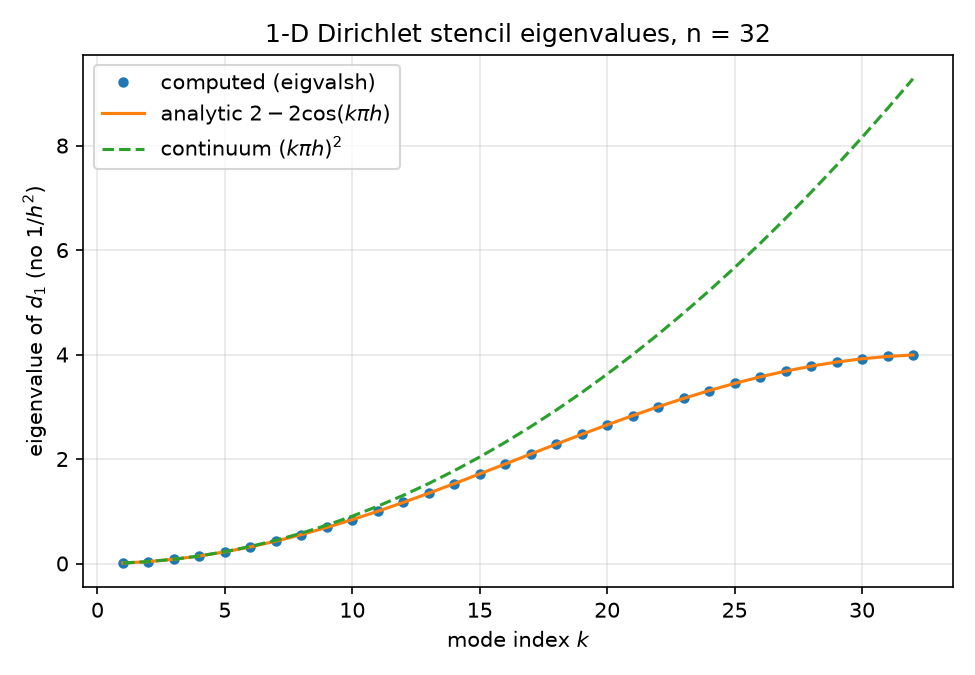 — computed dots sit exactly on the analytic $2 - 2\cos$ curve, and both peel away from the continuum parabola $(k\pi h)^2$ once $k\pi h$ is no longer small.
Spectral symmetry. Substituting $k \mapsto n+1-k$ gives $\cos!\big((n+1-k)\pi h\big) = \cos(\pi - k\pi h) = -\cos(k\pi h)$, hence
\[\lambda_{n+1-k} = 4 - \lambda_k .\]The 1-D spectrum is symmetric about $2$ (the diagonal entry). This innocuous identity has a 2-D consequence used in §5.
3. DST-I diagonalization and the fast Poisson solver
Orthogonality. Normalize the eigenvectors. Define the matrix
\[S_{jk} = \sqrt{\frac{2}{n+1}}\, \sin\!\left(\frac{jk\pi}{n+1}\right), \qquad 1 \le j, k \le n .\]This is the Discrete Sine Transform of type I (DST-I). The normalization comes from the discrete orthogonality relation
\[\sum_{j=1}^{n} \sin\!\left(\frac{jk\pi}{n+1}\right)\sin\!\left(\frac{jl\pi}{n+1}\right) = \frac{n+1}{2}\,\delta_{kl}, \qquad 1 \le k, l \le n,\]which follows from product-to-sum ($2\sin a \sin b = \cos(a-b) - \cos(a+b)$) and the closed geometric sum $\sum_{j=0}^{n} \cos\frac{jm\pi}{n+1} \in {0, 1}$ for integer $m \not\equiv 0 \pmod{2(n+1)}$; for $k = l$ the $\cos(a-b)$ term contributes $n$ ones and the correction terms assemble to $(n+1)/2$. (Alternatively: eigenvectors of a symmetric matrix with distinct eigenvalues are automatically orthogonal; the relation just fixes the norm.)
$S$ is symmetric ($S_{jk} = S_{kj}$ by inspection) and orthogonal, hence involutory:
\[S = S^{\mathsf T} = S^{-1}, \qquad S^2 = I .\]The eigendecomposition of the 1-D stencil is therefore
\[d_1 = S\, \Lambda\, S, \qquad \Lambda = \operatorname{diag}(\lambda_1, \dots, \lambda_n) .\]Fast Poisson solver. Because (a) $S$ diagonalizes $d_1$, (b) the 2-D operator is a Kronecker sum (§4), and (c) applying $S$ to a vector is a DST-I computable in $O(n\log n)$ via FFT (e.g. scipy.fft.dstn(..., type=1)), the exact solve $Au = b$ reduces to three passes:
$(S \otimes S)b$ is a DST-I applied along each of the two grid axes: $2n$ transforms of length $n$, total $O(n^2 \log n) = O(N \log N)$, versus $O(N \cdot n^2) = O(N^2)$ to factor with banded Cholesky (bandwidth $n = \sqrt{N}$; only its triangular solves are $O(N^{3/2})$), $O(N^{3/2})$ for sparse Cholesky with nested-dissection ordering, and $O(N \cdot \sqrt{\kappa}) = O(N^{3/2})$ for unpreconditioned CG (§6). This is the classical “fast Poisson solver,” and it is exact — no iteration at all. This repo deliberately does not implement it: the constant-coefficient Poisson problem here is a fully-instrumented testbed whose ground truth is knowable, used to study preconditioned Krylov methods that generalize to problems (like variable_poisson_2d, python/poisson.py lines 71–128) where no DST diagonalization exists. See 01-code-walkthrough.md.
4. Kronecker sums: the eigenpair theorem
The 2-D operator is assembled at python/poisson.py:67 as
\[A = \frac{1}{h^2}\left(d_1 \otimes I_n + I_n \otimes d_1\right),\]a Kronecker sum, often written $A = (d_1 \oplus d_1)/h^2$. The grid function $u(x_i, y_j)$ is flattened row-major with flat index $\;\mathtt{k} = i\cdot n + j$ (first axis slowest — matching Mathematica’s Flatten; see python/poisson.py lines 9–11), so kron(d1, I) differences along the $x$ (slow) axis and kron(I, d1) along $y$.
Theorem (Kronecker-sum eigenpairs). Let $B \in \mathbb{R}^{n\times n}$ have eigenpairs $(\mu_k, v^{(k)})$ and $C \in \mathbb{R}^{m\times m}$ have eigenpairs $(\nu_l, w^{(l)})$. Then
\[\left(B \otimes I_m + I_n \otimes C\right)\left(v^{(k)} \otimes w^{(l)}\right) = \left(\mu_k + \nu_l\right)\left(v^{(k)} \otimes w^{(l)}\right),\]and if ${v^{(k)}}$, ${w^{(l)}}$ are each complete (e.g. $B$, $C$ symmetric), the $nm$ vectors $v^{(k)} \otimes w^{(l)}$ form a complete eigenbasis, so $\operatorname{spec}(B \oplus C) = {\mu_k + \nu_l}$ with multiplicities counted over all pairs $(k,l)$.
Proof. Use the mixed-product identity $(B \otimes C)(x \otimes y) = Bx \otimes Cy$ (immediate from block structure: block $(i,i’)$ of $B\otimes C$ is $B_{ii’}C$, so row-block $i$ of $(B\otimes C)(x\otimes y)$ is $\sum_{i’} B_{ii’} x_{i’} \, C y = (Bx)_i \, Cy$). Then
\[(B \otimes I)(v \otimes w) = Bv \otimes w = \mu\,(v \otimes w), \qquad (I \otimes C)(v \otimes w) = v \otimes Cw = \nu\,(v \otimes w),\]and adding gives the claimed eigenrelation. For completeness: if ${v^{(k)}}{k=1}^n$ and ${w^{(l)}}{l=1}^m$ are orthonormal bases, then $\langle v^{(k)}\otimes w^{(l)},\, v^{(k’)}\otimes w^{(l’)}\rangle = \langle v^{(k)}, v^{(k’)}\rangle\,\langle w^{(l)}, w^{(l’)}\rangle = \delta_{kk’}\delta_{ll’}$, so the $nm$ tensor products are orthonormal, hence a basis of $\mathbb{R}^{nm}$. $\blacksquare$
Note the contrast with the Kronecker product: $\operatorname{spec}(B \otimes C) = {\mu_k \nu_l}$ (eigenvalues multiply); for the Kronecker sum they add. Same eigenvectors in both cases.
Applied to $A$. With $B = C = d_1$ and the $1/h^2$ scaling:
\[\boxed{\; \Lambda_{k,l} = \frac{\lambda_k + \lambda_l}{h^2} = \frac{4}{h^2}\left[\sin^2\!\left(\frac{k\pi h}{2}\right) + \sin^2\!\left(\frac{l\pi h}{2}\right)\right], \qquad V^{(k,l)}_{(i,j)} = \sin(k\pi x_i)\,\sin(l\pi y_j), \;}\]for $k, l = 1, \dots, n$ — the sampled continuum eigenfunctions $\sin(k\pi x)\sin(l\pi y)$, again exactly. The 2-D diagonalizer is $S \otimes S$ (2-D DST-I), which is what makes §3’s fast solver work.
Verification. python/experiments/spectra.py lines 67–74 forms all $1024$ tensor sums (eigs_d1_ana[:,None] + eigs_d1_ana[None,:]).ravel() / h**2, sorts, and compares against eigvalsh(A.toarray()): max deviation $2.73\times10^{-11}$ on eigenvalues of magnitude up to $8.7\times10^3$ (relative $\sim 3\times10^{-15}$, i.e. float64-exact). The independent Mathematica check mathematica/eigen_check.wls (lines 29–38) does the same with Eigenvalues and Outer[Plus, ...]. The sorted spectrum overlay is 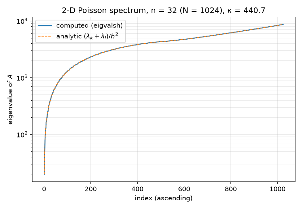 .
.
5. The spectrum of $A$: extremes, continuum limits, symmetry
At $n = 32$, $h = 1/33$, from results/spectra.json:
Smallest eigenvalue ($k = l = 1$):
\[\lambda_{\min}(A) = \frac{8}{h^2}\sin^2\!\left(\frac{\pi h}{2}\right) = 19.72430527164353 \quad\xrightarrow{h\to 0}\quad 2\pi^2 = 19.7392088\ldots\]The continuum limit is the fundamental Dirichlet eigenvalue $\pi^2(1^2 + 1^2) = 2\pi^2$ of $-\Delta$ on the unit square. The discrete deficit follows §2’s expansion:
\[\lambda_{\min}(A) = 2\pi^2\left(1 - \frac{(\pi h)^2}{12} + O(h^4)\right), \qquad \frac{(\pi h)^2}{12}\bigg\vert _{h = 1/33} = 7.55\times10^{-4},\]and indeed $(2\pi^2 - 19.72431)/2\pi^2 = 7.55\times10^{-4}$ — the standard $O(h^2)$ consistency of the 5-point stencil, visible here as an eigenvalue statement.
Largest eigenvalue ($k = l = n$). Using $\sin\frac{n\pi h}{2} = \sin!\big(\frac{\pi}{2} - \frac{\pi h}{2}\big) = \cos\frac{\pi h}{2}$:
\[\lambda_{\max}(A) = \frac{8}{h^2}\cos^2\!\left(\frac{\pi h}{2}\right) = 8692.275694728356 \quad\xrightarrow{h\to 0}\quad \frac{8}{h^2} = 8(n+1)^2 = 8712 .\]Unlike $\lambda_{\min}$, this does not converge to any continuum eigenvalue — it diverges as $8/h^2$, tracking the top of the discrete band ($4$ per dimension in stencil units, cf. Gershgorin: every disc is centered at $4/h^2$ with radius $\le 4/h^2$, so $\operatorname{spec}(A) \subset (0, 8/h^2)$). The highest mode is the checkerboard $\sin(n\pi x_i)\sin(n\pi y_j) = (\pm 1)^{i+j}\sin(\pi x_i)\sin(\pi y_j)$-modulated oscillation — pure grid-scale noise with no continuum counterpart.
Exact spectral symmetry. From §2’s identity $\lambda_{n+1-k} = 4 - \lambda_k$, the map $(k,l) \mapsto (n+1-k,\, n+1-l)$ sends
\[\Lambda_{k,l} \;\longmapsto\; \frac{8}{h^2} - \Lambda_{k,l},\]so the 2-D spectrum is exactly symmetric about its center $4/h^2 = 4(n+1)^2 = 4356$. Consequences checked in the results:
- $\lambda_{\min} + \lambda_{\max} = 19.724305\ldots + 8692.275694\ldots = 8712.000000 = 8/h^2$ exactly;
- the median eigenvalue of $A$ is exactly $4356.0$ (results/npo_spectrum.json,
eig_A.median); - the spectral density near the top edge mirrors the density near the bottom edge. Near the bottom, $\Lambda_{k,l} \approx \pi^2(k^2 + l^2)$, so the counting function $#{\Lambda \le \lambda} \approx \frac{\pi}{4} \cdot \frac{\lambda}{\pi^2}$ grows only linearly in $\lambda$ (quarter-disk area in $(k,l)$-space) — the band edges are sparse, and by symmetry so is the top. This “slow decay from the top” is exactly what defeats low-rank preconditioning in §8.3.
The semilog sorted spectrum shows both features: a steep initial rise (few small eigenvalues) followed by a long, slowly-climbing shoulder — by index 434 of 1024 the eigenvalues already exceed $4\times10^3$, i.e. within a factor $\sim 2.2$ of $\lambda_{\max}$.
6. Condition number: exact formula and $O(n^2)$ growth
Since $A$ is SPD, $\kappa_2(A) = \lambda_{\max}/\lambda_{\min}$, and both extremes share the factor $8/h^2$:
\[\kappa(A) = \frac{\sin^2(n\pi h/2)}{\sin^2(\pi h/2)} = \frac{\cos^2(\pi h/2)}{\sin^2(\pi h/2)} = \cot^2\!\left(\frac{\pi}{2(n+1)}\right).\]The $\sin^2$-ratio form is implemented in python/experiments/spectra.py lines 47–50 (kappa_analytic); the $\cot^2$ form is the one used by the independent Mathematica check (mathematica/eigen_check.wls:42, Cot[Pi/(2(n+1))]^2) — identical by the reflection $\sin(n\pi h/2) = \cos(\pi h/2)$. At $n = 32$:
agreeing to $3.3\times10^{-13}$ relative — every printed digit in both the Python and Mathematica runs.
Asymptotics. $\cot x = 1/x - x/3 + O(x^3)$, so with $x = \frac{\pi}{2(n+1)}$:
\[\kappa(A) = \frac{4(n+1)^2}{\pi^2} - \frac{2}{3} + O(n^{-2}) .\]At $n = 32$ the leading term is $4 \cdot 33^2/\pi^2 = 441.3551$ (results/spectra.json, kappa_asymptotic_4n1sq_over_pisq), overshooting the exact $440.6886$ by $0.667 \approx 2/3$ — the next Taylor coefficient, visible in the data.
$O(n^2)$ growth, from the exact formula (kappa_vs_n_analytic / kappa_over_nsq in results/spectra.json):
| $n$ | $\kappa(A)$ (exact) | $\kappa/n^2$ |
|---|---|---|
| 8 | 32.163 | 0.50255 |
| 16 | 116.461 | 0.45493 |
| 32 | 440.689 | 0.43036 |
| 64 | 1711.661 | 0.41789 |
| 128 | 6743.677 | 0.41160 |
$\kappa/n^2$ descends monotonically toward the limit $4/\pi^2 = 0.405285$ (the residual gap is the $(n+1)^2/n^2$ factor plus the $-2/3$ correction). The log-log plot 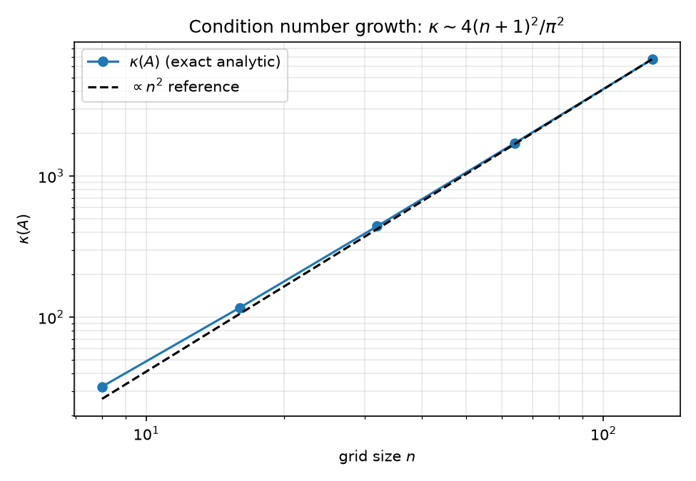 is parallel to the $n^2$ reference by $n = 32$.
What this costs CG. The classical CG bound (derived in 04-krylov-and-pcg.md) gives, in the $A$-norm,
\[\Vert e_j\Vert _A \le 2\left(\frac{\sqrt{\kappa}-1}{\sqrt{\kappa}+1}\right)^{j} \Vert e_0\Vert _A .\]With $\kappa = 440.689$: $\sqrt{\kappa} = 20.99$, contraction factor $\rho = 19.99/21.99 = 0.9091$, and reaching $10^{-10}$ needs at most $j \ge \ln(2\times10^{10})/\ln(1/\rho) \approx 23.72/0.09535 \approx 249$ iterations. Observed: 116 iterations to relative residual $6.667\times10^{-11}$ (results/results.json, canonical/cg_none) — about $2.1\times$ better than the worst-case bound, because CG is adaptive to the whole spectrum, not just its endpoints, and because the GRF right-hand side (03-gaussian-random-fields.md) concentrates energy in smooth modes. The scaling message stands: $\sqrt{\kappa} \propto n$, so unpreconditioned CG iterations grow linearly with grid refinement — halving $h$ doubles the iteration count, which is the entire motivation for the preconditioner studies in reports 05–07.
7. Verification summary (Python + Mathematica)
Two fully independent implementations check every formula above:
- Python (python/experiments/spectra.py,
uv run python python/experiments/spectra.py): builds $d_1$ and $A$ from python/poisson.py, runs densenumpy.linalg.eigvalsh, compares againstd1_eigs_analyticand the tensor-sum construction, and writes results/spectra.json plus the three figures. Deviations: $2.22\times10^{-15}$ (1-D), $2.73\times10^{-11}$ (2-D, few-ulp relative at eigenvalue magnitude $\sim10^4$). - Mathematica (mathematica/eigen_check.wls,
wolframscript -file mathematica/eigen_check.wls): rebuilds the sameSparseArray/KroneckerProductconstruction the Python port mirrors (the docstring at python/poisson.py lines 3–7 quotes it verbatim), checksEigenvalues[Normal[d1]]against2 - 2 Cos[k Pi/(n+1)],Eigenvalues[Normal[A]]againstOuter[Plus, ...] / h^2, and the condition number againstCot[Pi/(2(n+1))]^2— the trig-identity-transformed version of the Python formula, so agreement between the two scripts also validates the identity chain in §6.
8. What preconditioning does to this spectrum
PCG convergence is governed by the spectrum of the preconditioned operator $M^{-1}A$ (equivalently $M^{-1/2}AM^{-1/2}$ for SPD $M$) — both its condition number and its clustering. The spectrum derived above explains all four preconditioner outcomes in 08-results.md.
8.1 Jacobi: provably nothing (constant coefficients) — see 05-classical-preconditioners.md
Every diagonal entry of $A$ is $\Lambda$-independent: $A_{kk} = 4/h^2 = 4356$ (row sums of the two stencils). Jacobi preconditioning therefore sets $M = \frac{4}{h^2}I$, and $M^{-1}A = \frac{h^2}{4}A$ — a scalar rescaling, which changes no eigenvalue ratios and, since PCG is invariant under $M \mapsto cM$ in exact arithmetic, produces the same iterates up to floating-point roundoff. Measured: 116 iterations for both, final relative residuals agreeing to 15 significant digits ($6.666547523655469\times10^{-11}$ vs $\ldots465\times10^{-11}$, results/results.json), residual histories agreeing to $4.4\times10^{-16}$ (results/baseline.json). On variable_poisson_2d (diagonal jumping from $4356$ to $435{,}600$ with contrast 100) the diagonal does carry spectral information and Jacobi cuts $771 \to 137$ iterations — the spectrum-level story is in 05-classical-preconditioners.md.
8.2 ILU: spectrum collapsed — see 05-classical-preconditioners.md
Incomplete LU replaces the analysis above wholesale: $M^{-1}A \approx I$ + small perturbation, clustering essentially the entire spectrum near 1. Measured: 5 iterations (results/results.json, canonical/cg_ilu).
8.3 Nyström: defeated by the flat top — see 07-nystrom-preconditioning.md
The randomized Nyström preconditioner (Frangella–Tropp–Udell, arXiv:2110.02820) builds a rank-$\ell$ approximation $\hat A_\ell \approx U\hat\Lambda U^{\mathsf T}$ of the top of the spectrum and constructs $P$ so that $P^{-1}$ shrinks those top-$\ell$ directions down to the level $\hat\lambda_\ell$, leaving the orthogonal complement untouched. The best possible rank-$\ell$ outcome is therefore
\[\kappa_{\text{opt}}(\ell) = \frac{\lambda_{\ell+1}^{\downarrow}}{\lambda_{\min}},\]where $\lambda^{\downarrow}$ sorts descending. But §5 showed the counting function near the top edge is only linear — the eigenvalues of $A$ decay slowly from $\lambda_{\max}$. From results/nystrom.json (exact dense eigensolve of $P^{-1/2}AP^{-1/2}$, computed in python/experiments/run_nystrom.py lines 40–66 using the closed-form $P^{-1/2} = I + U(\sqrt{s}-1)U^{\mathsf T}$):
| rank $\ell$ | $\kappa(P^{-1/2}AP^{-1/2})$ | optimal $\kappa_{\text{opt}}(\ell) = \lambda^{\downarrow}{\ell+1}/\lambda{\min}$ | CG iterations |
|---|---|---|---|
| — (none) | 440.69 | — | 116 |
| 16 | 439.62 | 428.91 | 123 |
| 64 | 434.52 | 395.67 | 123 |
| 128 | 426.58 | 359.61 | 122 |
| 256 | 407.46 | 298.41 | 119 |
Even perfect deflation of the top 256 of 1024 eigenvalues (25% of the spectrum!) would leave $\kappa = 298.4$ — i.e. $\lambda^{\downarrow}{257} = 298.41 \times 19.724 \approx 5886$, still 68% of $\lambda{\max}$. The realized $\kappa$ values are worse still (sketching error), and the marginal $\kappa$ gain is outweighed by the sketch’s slight distortion of the rest of the spectrum: all Nyström variants take more iterations than plain CG (119–123 vs 116). The 2-D Laplacian, with its symmetric, edge-sparse, center-dense spectrum, is the adversarial case for a method designed for fast-decay/ridge-regularized spectra where $\lambda^{\downarrow}_{\ell+1}$ plunges to the regularization level within small $\ell$. Full discussion: 07-nystrom-preconditioning.md.
8.4 NPO: clustering without symmetry — see 06-neural-preconditioner.md
The neural preconditioner (NPO, arXiv:2502.01337) is a nonlinear map $r \mapsto \mathrm{NPO}(r)$, not an SPD matrix. Its column-wise linearization $\tilde M$ (assembled from 1024 canonical-basis applies, results/npo_spectrum.json) is markedly non-symmetric ($\Vert \tilde M - \tilde M^{\mathsf T}\Vert _F/\Vert \tilde M\Vert _F = 0.568$) and the operator is markedly nonlinear ($\Vert \tilde M b - \mathrm{NPO}(b)\Vert /\Vert \mathrm{NPO}(b)\Vert = 0.432$ on the canonical GRF $b$) — yet $\operatorname{eig}(\tilde M A)$ lands entirely in the right half-plane ($\operatorname{Re} \in [248.8,\, 3125.2]$, $\max\vert \operatorname{Im}\vert = 257.1$, zero non-positive real parts) and is tightly clustered: modulus spread $\max\vert \lambda\vert /\min\vert \lambda\vert = 12.56$ versus $\kappa(A) = 440.69$ ($35\times$ tighter), with 98.1% of eigenvalues within $[0.5, 2]\times$ the median versus 82.0% for $A$’s spectrum. Clustering — not symmetry — is what a flexible Krylov method can exploit: flexible PCG (Notay) converges in 30 iterations vs 116, while plain PCG (whose Fletcher–Reeves recursion assumes a fixed SPD $M$) stalls at $\sim10^{-5}$ and never converges (2000 iterations, deliberate negative control). See 06-neural-preconditioner.md and the FCG derivation in 04-krylov-and-pcg.md.
Summary of exact formulas
\[\begin{aligned} \operatorname{spec}(d_1) &: \quad \lambda_k = 2 - 2\cos\frac{k\pi}{n+1} = 4\sin^2\frac{k\pi}{2(n+1)}, \qquad v^{(k)}_j = \sin\frac{jk\pi}{n+1} \\[4pt] d_1 &= S\Lambda S, \qquad S_{jk} = \sqrt{\tfrac{2}{n+1}}\sin\tfrac{jk\pi}{n+1}, \qquad S = S^{\mathsf T} = S^{-1} \\[4pt] \operatorname{spec}(A) &: \quad \Lambda_{k,l} = \frac{\lambda_k + \lambda_l}{h^2}, \qquad V^{(k,l)} = v^{(k)} \otimes v^{(l)}, \qquad \text{diagonalizer } S \otimes S \\[4pt] \lambda_{\min}(A) &= \tfrac{8}{h^2}\sin^2\tfrac{\pi h}{2} \to 2\pi^2, \qquad \lambda_{\max}(A) = \tfrac{8}{h^2}\cos^2\tfrac{\pi h}{2} \to \tfrac{8}{h^2}, \qquad \lambda_{\min} + \lambda_{\max} = \tfrac{8}{h^2} \\[4pt] \kappa(A) &= \cot^2\frac{\pi}{2(n+1)} = \frac{4(n+1)^2}{\pi^2} - \frac{2}{3} + O(n^{-2}) \quad\Rightarrow\quad \text{CG iterations} \propto \sqrt{\kappa} \propto n . \end{aligned}\]Every one of these is confirmed to float64 precision at $n = 32$ by results/spectra.json and mathematica/eigen_check.wls.