03 — The Gaussian-Random-Field Right-Hand Side
Every experiment in this repo solves $Ax=b$ with the same right-hand side family: a mean-zero Gaussian random field (GRF) with Matérn-type power spectrum, synthesized spectrally via the FFT. This report derives the construction line by line, explains the two non-obvious design choices (the * n frequency scaling and the Re(IFFT) of non-Hermitian complex noise), gives the Matérn-covariance interpretation of $(\alpha, \tau)$, and quantifies the torus-vs-Dirichlet-box mismatch.
Code under discussion:
- Python:
grf_rhsin python/poisson.py (def at line 131; the whole computation is lines 176–184 — seven statements). - Mathematica reference: mathematica/poisson_pcg.wls lines 40–47.
Context: this GRF family is the de-facto standard data distribution for neural-operator PDE benchmarks. The FNO paper (Li et al., Fourier Neural Operator for Parametric PDEs, ICLR 2021, arXiv:2010.08895) builds its Darcy coefficients on the base GRF $\mathcal N!\big(0,(-\Delta+9I)^{-2}\big)$ — exactly $\alpha=2,\tau=3$ in the notation below — though the coefficients themselves are the pushforward $\psi_#\,\mathcal N\big(0,(-\Delta+9I)^{-2}\big)$ of that field through a binary threshold map (so they are piecewise-constant, not Gaussian). The NPO paper (arXiv:2502.01337, Sec. 5.1.2) says only that its right-hand sides are sampled “from a Gaussian Random Field (GRF)” mapped onto the same mesh as $A$ — it does not specify the spectrum or the sampling method. The defaults alpha=2.0, tau=3.0 in grf_rhs follow the FNO convention as the concrete instantiation of that underspecified choice. See 06-neural-preconditioner.md for how 40 draws of this field (seeds 100–139) form the NPO training set, and 08-results.md for everything solved against the canonical seed-42 draw.
1. The pipeline at a glance
Mathematica (poisson_pcg.wls L40–47):
alpha = 2.0; tau = 3.0;
freqs    = N@RotateRight[Range[-n/2, n/2 - 1], n/2]*n;
spectrum = 1.0/(Outer[Plus, freqs^2, freqs^2] + tau^2)^(alpha/2.0);
SeedRandom[42];
noise    = RandomVariate[NormalDistribution[], {n, n, 2}] . {1, I};
grfRaw   = Re@InverseFourier[noise*spectrum, FourierParameters -> {-1, -1}];
b        = Standardize@Flatten@grfRaw;
Python port (python/poisson.py L176–184):
f = np.roll(np.arange(-n // 2, n // 2), n // 2) * n
spectrum = 1.0 / (f[:, None] ** 2 + f[None, :] ** 2 + tau**2) ** (alpha / 2.0)

rng = np.random.default_rng(seed)
noise = rng.standard_normal((n, n, 2)) @ np.array([1.0, 1.0j])
field = np.real(np.fft.ifft2(noise * spectrum))

flat = field.ravel()  # row-major, matching Mathematica Flatten
return (flat - flat.mean()) / flat.std(ddof=1)
In math: with $k=(k_1,k_2)\in{-n/2,\dots,n/2-1}^2$ integer wavenumbers,
\[b(x) \;\propto\; \operatorname{Re}\!\Big[\sum_{k} \underbrace{\big(n^2\vert k\vert ^2+\tau^2\big)^{-\alpha/2}}_{S_k}\, Z_k\, e^{2\pi i\, k\cdot x/n}\Big], \qquad Z_k = G^{(1)}_k + i\,G^{(2)}_k,\;\; G^{(j)}_k \overset{iid}{\sim}\mathcal N(0,1),\]followed by exact removal of the spatial mean and rescaling to unit sample variance. Sections 2–6 unpack each factor.
The port is distribution-exact but not draw-exact: NumPy’s PCG64 stream under default_rng(42) cannot bit-match Mathematica’s SeedRandom[42] stream, so figures/grf_field.png and figures/mma_source_grf.png show two different samples of the same distribution. That is fine for the experiments — each language’s suite is internally self-consistent — but it is why the two figures don’t look identical.
2. The frequency grid: fftshifted ordering and the * n scaling
2.1 Ordering
Range[-n/2, n/2-1] is $[-16,\dots,15]$ for $n=32$; RotateRight[..., n/2] cyclically shifts by 16, giving
— exactly the standard DFT ordering (DC in slot 0, positive frequencies first, then negatives), i.e. the inverse of fftshift. NumPy reproduces it with np.roll(np.arange(-n//2, n//2), n//2) (poisson.py L176); it equals np.fft.fftfreq(n) * n. This ordering is mandatory because ifft2 (and InverseFourier) index Fourier coefficients in DFT order — building spectrum on a shifted grid without unshifting would scramble which noise mode gets which amplitude. Verified numerically: the array starts [0, 32, 64, ...] and ends [..., -64, -32] after the * n scaling, with the unpaired Nyquist frequency $-n/2$ sitting at index 16 (f[16] = -512).
2.2 What the * n actually does
After scaling, the spectral amplitude at integer mode $k$ is
\[S_k = \big(n^2 k_1^2 + n^2 k_2^2 + \tau^2\big)^{-\alpha/2} = n^{-\alpha}\Big(\vert k\vert ^2 + \big(\tfrac{\tau}{n}\big)^2\Big)^{-\alpha/2}.\]Two consequences, one trivial and one substantive:
- The prefactor $n^{-\alpha}$ is irrelevant. It is a global constant, annihilated by the final standardization (Sec. 6).
- The effective mass parameter is $\tau_{\mathrm{eff}}=\tau/n = 3/32 = 0.09375$, not $\tau=3$. The Matérn “knee” — the wavenumber below which the spectrum flattens — sits at $\vert k\vert \approx\tau_{\mathrm{eff}}\approx 0.094$, below the first resolvable nonzero mode $\vert k\vert =1$. So on every mode the field actually contains, the spectrum is a nearly pure power law $\vert k\vert ^{-\alpha}$: the relative flattening at $k=(1,0)$ is $\tau^2/n^2 = 9/1024 \approx 0.88\%$. Concretely (verified): $S_{(0,1)}/S_{(0,2)} = 3.974$ versus exactly $4$ for a pure $\vert k\vert ^{-2}$ law.
Compare the FNO-paper normalization, which uses angular wavenumbers: amplitude $\propto(4\pi^2\vert k\vert ^2+\tau^2)^{-\alpha/2}$, i.e. $\tau_{\mathrm{eff}} = \tau/2\pi \approx 0.477$ and a $\tau^2/4\pi^2 \approx 23\%$ flattening at mode 1. The * n convention here (with $n=32 \approx 5.1\times 2\pi$) therefore produces a smoother, longer-range field than FNO’s at the same $(\alpha,\tau)$ — effectively scale-free across the resolved band. Same family, slightly different point in it; nothing downstream depends on this distinction since every experiment uses the one convention consistently.
The DC entry $S_{(0,0)} = \tau^{-\alpha} = 1/9 \approx 0.1111$ is enormous relative to its neighbors — $S_{(0,0)}/S_{(0,1)} = (n^2+\tau^2)/\tau^2 \cdot \ldots = 1033/9 = 114.8$ in amplitude, and the DC mode carries $99.95\%$ of the raw spectral energy $\sum_k S_k^2$ (verified: $\sum S_k^2 = 1.2351\times10^{-2}$, of which $S_{(0,0)}^2 = 1/81 = 1.2346\times10^{-2}$). This would be alarming except that a DC Fourier mode is a spatial constant, and Standardize subtracts the sample mean — which for a band-limited periodic field equals the DC component exactly (Sec. 6). So the huge DC amplitude is created and then exactly destroyed; only the $\vert k\vert \ge 1$ modes survive into $b$.
3. The power spectrum as a Matérn covariance
3.1 Covariance operator
A mean-zero Gaussian field with Fourier amplitudes $S_k \propto (\vert k\vert ^2+\tau^2)^{-\alpha/2}$ has power spectral density $S_k^2 \propto (\vert k\vert ^2+\tau^2)^{-\alpha}$, i.e. covariance operator
\[C = \sigma^2\big({-\Delta} + \tau^2 I\big)^{-\alpha}\]on the torus (where $-\Delta$ has Fourier symbol $\vert k\vert ^2$ in the wavenumber units used — with the code’s * n scaling the symbol is $n^2\vert k\vert ^2$, which just rescales $\tau$ per Sec. 2.2). This is exactly the base measure $\mu = \mathcal N\big(0, (-\Delta + 9I)^{-2}\big)$ that the FNO paper pushes through a threshold map to make its Darcy coefficients; the NPO paper (Sec. 5.1.2) specifies only an unqualified “Gaussian Random Field” for its right-hand sides.
3.2 Whittle–Matérn dictionary
The Whittle–Matérn covariance in $d$ dimensions with smoothness $\nu$ and inverse length-scale $\tau$ has spectral density
\[\hat C(\xi) \;\propto\; \big(\vert \xi\vert ^2 + \tau^2\big)^{-(\nu + d/2)},\]so matching exponents gives
\[\boxed{\;\nu = \alpha - \tfrac{d}{2}\;}\qquad\Rightarrow\qquad \nu = 2 - 1 = 1 \;\text{ for }\; \alpha=2,\ d=2 .\]Interpretation of the two knobs:
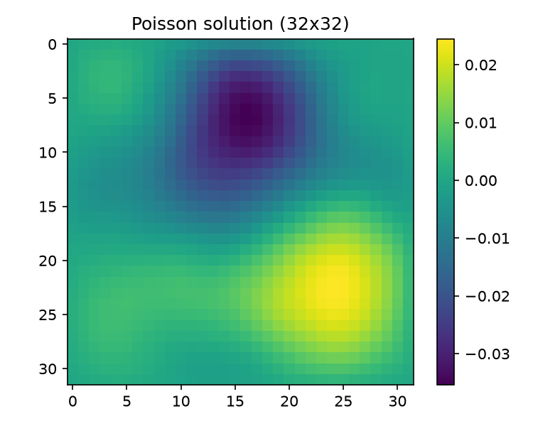
- $\alpha$ controls smoothness. Sobolev regularity of samples: $\mathbb E\,\Vert b\Vert _{H^s}^2 \propto \sum_k (1+\vert k\vert ^2)^s (\vert k\vert ^2+\tau^2)^{-\alpha} < \infty \iff 2(\alpha - s) > d$, i.e. samples lie a.s. in $H^s$ for every $s < \alpha - d/2 = 1$ and not in $H^1$. Equivalently Matérn $\nu=1$: continuous, but not mean-square differentiable (that requires $\nu>1$). By elliptic regularity the exact solution $u = A^{-1}b$ then sits (formally, modulo box-corner caveats) two derivatives higher, in $H^{3-\varepsilon}$ — a smooth-looking blob, cf. figures/solution_field.png.
- $\tau$ controls correlation length, roughly $\ell \sim 1/\tau_{\mathrm{eff}}$ in domain units. With the code’s $\tau_{\mathrm{eff}} = \tau/n \approx 0.094 \ll 1$ the correlation length exceeds the domain: the field is dominated by its few lowest modes.
3.3 Measured correlation structure (seed-42 draw, $n=32$)
From the exact covariance formula of Sec. 4, the theoretical lag-1 (one grid cell) correlation after DC removal is $0.9698$; matching sample statistics from the actual grf_rhs(32) draw:
| quantity | value |
|---|---|
| corr(row 0, row 16) — half-domain separation | $0.330$ |
| corr(row 0, row 31) — wrap-around neighbors on the torus | $0.972$ |
| $\min b$, $\max b$ (after standardization) | $-3.200$, $+2.283$ |
| sample mean, sample std (ddof=1) | $2.8\times10^{-17}$, $1.000000$ |
The $0.972$ wrap-around correlation is the periodicity artifact discussed in Sec. 7.
Why this matters for the solver benchmarks: a $\vert k\vert ^{-\alpha}$-weighted $b$ concentrates energy in the low end of $A$’s spectrum — precisely the eigenmodes CG resolves last (see 02-eigenvalues.md for the eigenstructure and 04-krylov-and-pcg.md for the convergence consequences). A white-noise $b$ would flatter the solvers; the GRF is the harder and more physical choice, and it is what the neural preconditioner is trained on, so train/test distributions match by construction.
4. Complex white noise and why Re(IFFT) of non-Hermitian noise is legitimate
4.1 The construction
rng.standard_normal((n, n, 2)) @ [1, 1j] (poisson.py L180) builds
a circularly-symmetric complex Gaussian array: $\mathbb E[Z_k \bar Z_l] = 2\,\delta_{kl}$ and, crucially, vanishing pseudo-covariance $\mathbb E[Z_k Z_l] = 0$. Note what it is not: it is not Hermitian-symmetric ($Z_{-k} \ne \bar Z_k$), so ifft2(noise * spectrum) is a genuinely complex field, and the code simply takes its real part (L181).
A textbook spectral sampler instead enforces $Z_{-k}=\bar Z_k$ (with real DC and Nyquist modes) so the IFFT is real by construction. The Re shortcut skips all of that bookkeeping — including the fiddly special-casing of the self-conjugate modes $k\in{0,n/2}^2$ (recall the unpaired Nyquist frequency at index $n/2$, Sec. 2.1). The question is whether the result is still a stationary GRF with the right spectrum.
4.2 Derivation: it is, with exactly half the variance
Write the complex field ($\mathcal F^{-1}$ = ifft2, kernel $e^{+2\pi i k\cdot x/n}$, prefactor $1/n^2$):
Using $\operatorname{Re}a = \tfrac12(a+\bar a)$ and the two moment identities ($\mathbb E[Z_k\bar Z_l]=2\delta_{kl}$, $\mathbb E[Z_kZ_l]=0$):
\[\mathbb E\big[F(x)\overline{F(y)}\big] = \frac{2}{n^4}\sum_k S_k^2\, e^{2\pi i k\cdot(x-y)/n}, \qquad \mathbb E\big[F(x)F(y)\big] = \frac{1}{n^4}\sum_k S_k^2\,\mathbb E[Z_k^2]\,e^{\cdots} = 0 .\]Because $S_k$ depends on $k$ only through $\vert k\vert ^2$ (with the wrapped DFT frequencies, $f_j^2 = f_{n-j}^2$), the first sum is invariant under $k\to -k$ and hence real. Expanding $\operatorname{Re}F(x)\operatorname{Re}F(y) = \tfrac14(F(x)+\bar F(x))(F(y)+\bar F(y))$ and using both identities:
\[\operatorname{Cov}\big(b_{\text{raw}}(x),\, b_{\text{raw}}(y)\big) = \tfrac12 \operatorname{Re}\,\mathbb E\big[F(x)\overline{F(y)}\big] = \frac{1}{n^4}\sum_k S_k^2 \cos\!\big(2\pi k\cdot(x-y)/n\big).\]This depends on $x-y$ only — stationary on the torus — and equals exactly half the covariance of the full complex field, which is the covariance a Hermitian-symmetrized sampler would deliver. The same computation for the cross-moment gives $\mathbb E[\operatorname{Re}F(x)\operatorname{Im}F(y)] = -\tfrac12\operatorname{Im}\mathbb E[F(x)\overline{F(y)}] = 0$ (the expectation is real), so $\operatorname{Re}F$ and $\operatorname{Im}F$ are jointly Gaussian and uncorrelated, hence independent iid copies of the same GRF. Taking the real part doesn’t distort anything; it merely discards an independent duplicate sample, at the cost of a factor $\tfrac12$ in variance — and that factor is a global constant erased by Standardize one line later, so it is exactly harmless.
Monte-Carlo verification (400 fresh draws, $n=32$, seeds 1000–1399 via np.random.default_rng(1000+k), averaging the spatial variance of each draw):
| quantity | theory | measured |
|---|---|---|
| per-point variance of $\operatorname{Re}F$ after mean removal, $\big(\sum_k S_k^2 - S_0^2\big)/n^4$ | $5.399\times10^{-12}$ | $5.59\times10^{-12}$ |
| spatial variance of $\operatorname{Im}F$ | same | $5.21\times10^{-12}$ |
| $\mathbb E\,\overline{\vert F\vert ^2}$ vs $2\times$ Re-variance incl. DC ($2\sum S_k^2/n^4 = 2.356\times10^{-8}$) | $2.356\times10^{-8}$ | $2.418\times10^{-8}$ |
| lag-$(0,1)$ correlation | $0.9698$ | $0.972$ (seed-42 sample) |
5. FFT-normalization equivalence: Mathematica vs NumPy
Mathematica’s InverseFourier[..., FourierParameters -> {-1, -1}] uses the kernel $e^{+2\pi i k\cdot x/n}$ with no prefactor; NumPy’s ifft2 uses the same kernel with prefactor $1/n^2$. The two transforms of the same input therefore differ by the constant factor $n^2 = 1024$ — nothing else (both docstring-documented in poisson.py L152–157 and verified by the conventions above). Since the very next operation standardizes the field (Sec. 6), this constant is unobservable, exactly like the $n^{-\alpha}$ from Sec. 2.2 and the $\tfrac12$ from Sec. 4.2. Any overall multiplicative normalization anywhere in the pipeline is a no-op. The only things that matter are the shape of $S_k$ over $k\ne 0$ and the noise distribution.
This is also why the FNO reference implementation’s amplitude prefactor $\sigma = \tau^{\frac12(2\alpha-d)}$ (their normalization to unit-ish marginal variance) has no counterpart here: Standardize performs the same role empirically, per sample.
6. What Standardize does
Mathematica Standardize[list] computes $(x - \bar x)/s$ with $s$ the sample standard deviation (Bessel-corrected); the Python port matches with ddof=1 (poisson.py L184). Three precise effects:
- Exact DC surgery. For a band-limited periodic field, the spatial mean over one full period equals the DC Fourier component: every $k\ne0$ mode integrates to zero exactly over the $n\times n$ grid, so $\overline{b_{\text{raw}}} = \operatorname{Re}(Z_0)\,S_0/n^2$. (Verified:
field.mean() == noise[0,0].real * S[0,0] / n**2to float precision.) Mean subtraction therefore zeroes the $k=0$ mode exactly and touches nothing else — the clean answer to the scary-looking $99.95\%$-of-energy DC mode from Sec. 2.2. - Scale fixing. Division by the sample std maps every draw to sample variance 1 (measured on seed 42: mean $2.8\times10^{-17}$, std $1.000000$), making all the dropped constants ($n^{-\alpha}$, $n^2$, $\tfrac12$) moot and giving every solver run a right-hand side with $\Vert b\Vert _2 = \sqrt{n^2-1}\approx 32.0$ regardless of $(\alpha,\tau)$ bookkeeping.
- A pedantic caveat. Normalizing by the per-sample std makes the resulting $b$ very slightly non-Gaussian (its marginal law is a Gaussian conditioned on its own empirical variance). With $n^2 = 1024$ weakly-correlated-ish degrees of freedom this is negligible, and it is standard practice in the benchmark literature; it just means “GRF” is accurate to first order, not a theorem, after this line.
Finally Flatten / .ravel() produce the row-major vector with flat index $k = i\,n + j$ — the same convention used to assemble $A$ from Kronecker products (see 01-code-walkthrough.md), so no transposition bug is possible between $b$ and $A$.
7. Torus sample, Dirichlet box: the deliberate mismatch
The sampler lives on the periodic torus: an $n\times n$ FFT grid, stationary covariance in $x-y$ mod $n$. The Poisson problem lives on the open unit square with homogeneous Dirichlet BCs, interior nodes $x_i = ih$, $h = 1/(n+1)$ (see 02-eigenvalues.md). Two consequences:
- Wrap-around correlation. Opposite edges of the sampled field are near-duplicates: corr(row 0, row 31) $= 0.972$ on the canonical draw — they are lag-1 neighbors on the torus. Visually, figures/grf_field.png tiles seamlessly; the color field “wants” to continue periodically. A field drawn from the honest Matérn measure on the box (e.g. via a KL expansion in the Dirichlet or Neumann eigenbasis of the Laplacian, as in the FNO paper’s Darcy setup) would have no such edge-to-edge coupling.
- Grid mismatch, cosmetic. The torus grid has $n$ points at spacing $1/n$; the Dirichlet interior grid has $n$ points at spacing $1/(n+1)$ shifted off the boundary. The code ignores this entirely and simply reinterprets the $n^2$ torus samples as nodal values of $b$ on the interior grid.
Neither point is a bug for this repo’s purpose. The right-hand side of a linear-solver benchmark is just data — any fixed $b$ defines a valid SPD system, and restricting a stationary Gaussian field to a sub-grid yields a perfectly valid (still Gaussian, still stationary as a process) vector. What is lost is only the interpretation of $b$ as a sample from the Matérn field naturally associated with the Dirichlet box, plus literal independence between values near opposite edges. What is gained is a seven-statement sampler, exact spectral control, and — most importantly — exact train/test consistency within this repo: the NPO paper (arXiv:2502.01337, Sec. 5.1.2) says only that right-hand sides are GRF samples mapped onto the mesh, so this repo fixes the FNO-style spectral sampler as its concrete instantiation and uses it everywhere. The NPO training pipeline draws from it (python/neural/train_npo.py L51–52 and L89: NUM_RHS = 40 fields, grf_rhs(32, alpha=2.0, tau=3.0, seed=100+k)), and the canonical evaluation $b$ is grf_rhs(32, ..., seed=42) everywhere (run_all.py L110, run_baseline.py L37, run_nystrom.py L72, eval_npo.py L43, npo_spectrum.py L51).
8. Figures
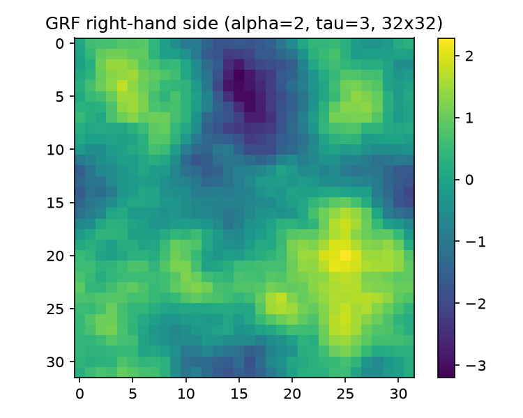
Python draw (np.random.default_rng(42)), rendered by run_baseline.py L79–89. A few large low-frequency blobs of both signs (dark top-center, bright lower-right), each spanning an $O(1)$ fraction of the domain — the visual signature of $\tau_{\mathrm{eff}}\ll 1$ (Sec. 2.2). Range after standardization: $[-3.20,\,2.28]$.
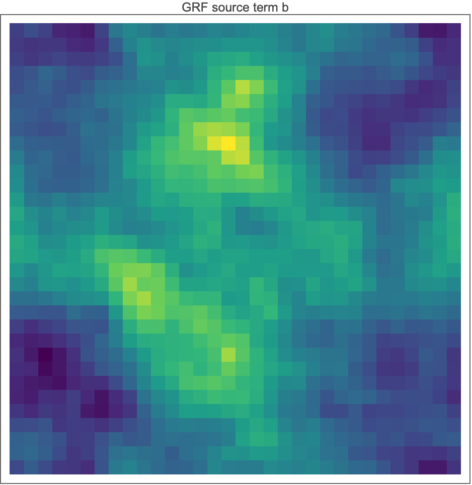
Mathematica draw (SeedRandom[42]), rendered by poisson_pcg.wls L99–102. Same distribution, different RNG stream, hence a different sample — the smoothness, large-blob character, and periodic-tiling tendency match the Python draw, which is the meaningful check.
9. Summary of verified facts
| claim | value / status |
|---|---|
DFT frequency ordering after RotateRight/np.roll |
$[0,1,\dots,15,-16,\dots,-1]$, Nyquist $-16$ at index 16 |
effective mass after * n scaling |
$\tau_{\mathrm{eff}} = \tau/n = 0.09375$; power-law deviation at mode 1 is $\tau^2/n^2 = 0.88\%$ ($S_{(0,1)}/S_{(0,2)}=3.974$ vs 4) |
| DC amplitude / energy | $S_{(0,0)} = 1/9$; ratio to first mode $114.8$; $99.95\%$ of $\sum S_k^2$; removed exactly by mean subtraction (spatial mean $\equiv$ DC coefficient, verified) |
| Matérn parameters at defaults | covariance $\propto(-\Delta+\tau^2)^{-\alpha}$, $\nu = \alpha - d/2 = 1$; $b\in H^{1-\varepsilon}$ a.s., $u\in H^{3-\varepsilon}$ |
Re(IFFT) of circular non-Hermitian noise |
stationary GRF with exactly $\tfrac12$ the Hermitian-sampler covariance; Im part is an independent iid copy; MC-verified (theory $5.40\times10^{-12}$ vs measured $5.59\times10^{-12}$ per-point variance, 400 draws) |
| FFT normalization | Mathematica {-1,-1} vs np.fft.ifft2 differ by the constant $n^2$; erased by Standardize, as are $n^{-\alpha}$ and $\tfrac12$ |
Standardize |
mean 0, sample std 1 (ddof=1); seed-42 draw: mean $2.8\times10^{-17}$, std $1.000000$, range $[-3.200, 2.283]$ |
| torus artifact | corr(row 0, row 31) $= 0.972$; harmless for solver benchmarking, standard in the neural-operator benchmark literature (e.g. FNO) |
| Python vs Mathematica draws | distribution-identical, not bit-identical (different RNG streams) |