04 — Krylov Subspaces and (Preconditioned) Conjugate Gradients
This report derives everything the repo’s solver layer does: the conjugate gradient method as $A$-norm minimization over Krylov subspaces, the exact 5-line state recurrence implemented in python/pcg.py and why it is a line-for-line match of the Mathematica pcgStep in mathematica/poisson_pcg.wls, preconditioning as a change of inner product, the $\sqrt{\kappa}$ Chebyshev convergence bound checked against the measured iteration counts, the scale-invariance of PCG in the preconditioner (which is why Jacobi is exactly plain CG on the canonical problem), and the flexible-CG (Polak–Ribière) variant that the nonlinear neural preconditioner requires.
Siblings: 01-code-walkthrough.md, 02-eigenvalues.md (spectrum of $A$), 03-gaussian-random-fields.md (the RHS), 05-classical-preconditioners.md, 06-neural-preconditioner.md, 07-nystrom-preconditioning.md, 08-results.md.
The concrete system throughout (from results/results.json config): $A = \texttt{poisson_2d}(32)$, the 5-point Dirichlet Laplacian on a $32\times 32$ interior grid, $N = n^2 = 1024$, $h = 1/33$; $b = \texttt{grf_rhs}(32, \alpha{=}2, \tau{=}3, \text{seed}{=}42)$; stopping rule $\Vert r_k\Vert 2/\Vert b\Vert _2 \le 10^{-10}$, maxiter 2000, $x_0 = 0$. From results/spectra.json: $\lambda{\min}(A) = 19.7243$, $\lambda_{\max}(A) = 8692.28$, $\kappa(A) = 440.6886$ (dense eigensolve and the analytic formula $\sin^2(n\pi h/2)/\sin^2(\pi h/2)$ agree to all printed digits — see 02-eigenvalues.md).
1. Krylov subspaces
For $Ax = b$ with $x_0 = 0$ (so $r_0 = b$), the $k$-th Krylov subspace is
\[\mathcal{K}_k(A, b) \;=\; \operatorname{span}\{\,b,\; Ab,\; A^2 b,\; \dots,\; A^{k-1} b\,\}.\]Why this space? Because $A^{-1}b$ is itself a polynomial in $A$ applied to $b$: if $q_A(\lambda) = \prod_{j}(\lambda - \lambda_j)$ is the minimal polynomial of $A$ restricted to the invariant subspace containing $b$ (degree $d$ = number of distinct eigenvalues with nonzero component in $b$), then $q_A(A)b = 0$ rearranges to
\[A^{-1} b \;=\; -\frac{1}{q_A(0)}\Big( A^{d-1} b + c_{d-1} A^{d-2} b + \dots + c_1 b \Big) \;\in\; \mathcal{K}_d(A, b),\]with $q_A(0) \ne 0$ since $A$ is SPD. So Krylov methods are polynomial methods: any iterate $x_k \in \mathcal{K}k$ can be written $x_k = q{k-1}(A)\, b$ for a polynomial $q_{k-1}$ of degree $\le k-1$, and the residual is
\[r_k \;=\; b - A x_k \;=\; \big(I - A\,q_{k-1}(A)\big)\, b \;=\; p_k(A)\, b, \qquad p_k(0) = 1,\ \deg p_k \le k .\]Every Krylov solver is a rule for choosing the residual polynomial $p_k$ subject to the normalization $p_k(0)=1$.
Finite termination. In exact arithmetic, CG terminates in at most $d$ = (number of distinct eigenvalues of $A$ represented in $b$) iterations. For our $A$ the eigenvalues are $(\lambda^{(1)}_k + \lambda^{(1)}_l)/h^2$ with $\lambda^{(1)}_k = 2 - 2\cos\frac{k\pi}{n+1}$ (02-eigenvalues.md); the sum is symmetric in $(k,l)$, so there are at most $n(n+1)/2 = 528$ distinct values in a space of dimension $1024$. This already halves the trivial termination bound — and it is a first hint that convergence is governed by the distribution of eigenvalues, not just their extremes. In practice CG reached $10^{-10}$ in 116 iterations, far below 528, for reasons quantified in §5.
2. CG as $A$-norm minimization
$A$ SPD defines the inner product $\langle u, v\rangle_A = u^{\top} A v$ and the energy norm $\Vert u\Vert _A = \sqrt{u^{\top} A u}$. Let $x^\star = A^{-1}b$ and $e = x^\star - x$. Minimizing the quadratic
\[\phi(x) \;=\; \tfrac12 x^{\top} A x - b^{\top} x \;=\; \tfrac12 \Vert x - x^\star\Vert _A^2 \;-\; \tfrac12 \Vert x^\star\Vert _A^2\]is equivalent to minimizing $\Vert e\Vert _A$. CG is defined by
\[x_k \;=\; \operatorname*{arg\,min}_{x \in \mathcal{K}_k(A,b)} \;\Vert x - x^\star\Vert _A .\]2.1 Optimality $\Leftrightarrow$ Galerkin orthogonality
$x_k$ is the $A$-orthogonal projection of $x^\star$ onto $\mathcal{K}_k$, i.e.
\[\langle x^\star - x_k,\; v\rangle_A = 0 \quad \forall v \in \mathcal{K}_k \qquad\Longleftrightarrow\qquad r_k = A(x^\star - x_k) \;\perp\; \mathcal{K}_k .\]Since $r_k \in \mathcal{K}{k+1}$ (it is $p_k(A)b$) and $r_k \perp \mathcal{K}_k$, the residuals ${r_0, \dots, r{k}}$ are mutually orthogonal and form an orthogonal basis of $\mathcal{K}_{k+1}$.
2.2 Why a short recurrence exists
Expand $x_{k+1} = x_k + \sum_{i\le k}\gamma_i p_i$ over any basis ${p_i}$ of $\mathcal{K}_{k+1}$ that is $A$-conjugate ($p_i^{\top} A p_j = 0$, $i\ne j$). Conjugacy decouples the minimization: each coefficient is a 1-D exact line search independent of the others,
\[\gamma_i \;=\; \frac{p_i^{\top} r_k}{p_i^{\top} A p_i},\]and Galerkin orthogonality makes $p_i^{\top} r_k = 0$ for all $i < k$ — so only one new coefficient per step survives. The deep structural reason a conjugate basis can itself be built with a short recurrence is symmetry of $A$: the Lanczos process $A V_k = V_{k+1} \tilde{T}_k$ produces a tridiagonal $T_k$ when $A = A^{\top}$ (a Hessenberg matrix that is also symmetric), so orthogonalizing $A p_k$ against all previous directions reduces to orthogonalizing against the last one. CG is exactly the LDL$^\top$ factorization of that tridiagonal system, giving the coupled two-term recurrences:
\[\boxed{ \begin{aligned} \alpha_k &= \frac{r_k^{\top} r_k}{p_k^{\top} A p_k}, & x_{k+1} &= x_k + \alpha_k p_k, & r_{k+1} &= r_k - \alpha_k A p_k, \\[2pt] \beta_k &= \frac{r_{k+1}^{\top} r_{k+1}}{r_k^{\top} r_k}, & p_{k+1} &= r_{k+1} + \beta_k p_k, & p_0 &= r_0 = b . \end{aligned}}\]Derivation of the two formulas:
- $\alpha_k$ (exact line search): $\frac{d}{d\alpha}\phi(x_k + \alpha p_k) = 0 \Rightarrow \alpha_k = \frac{p_k^{\top} r_k}{p_k^{\top} A p_k}$; then $p_k^{\top} r_k = (r_k + \beta_{k-1} p_{k-1})^{\top} r_k = r_k^{\top} r_k$ using $p_{k-1} \perp r_k$.
- $\beta_k$ (one-step $A$-conjugacy): require $p_{k+1}^{\top} A p_k = 0$ with $p_{k+1} = r_{k+1} + \beta_k p_k$:
where the second equality substitutes $A p_k = (r_k - r_{k+1})/\alpha_k$. The middle expression is the Polak–Ribière form, the right one the Fletcher–Reeves form; they coincide only because $r_{k+1}^{\top} r_k = 0$, which is a global consequence of running exact CG with a fixed operator. Keep this in mind — §6 shows the two forms diverge, catastrophically, when the preconditioner is nonlinear.
An induction (Saad, Iterative Methods for Sparse Linear Systems, 2nd ed., §6.7) confirms that these local conditions propagate globally: $r_i^{\top} r_j = 0$ and $p_i^{\top} A p_j = 0$ for all $i \ne j$, so the greedy one-step construction achieves the global $A$-norm minimum over $\mathcal{K}_k$ — the defining miracle of CG.
3. The implementation, and the exact match with Mathematica
3.1 The 5-line state recurrence
python/pcg.py lines 67–79 (the loop body of pcg) implement the preconditioned version of the boxed recurrence, with $z = M(r)$ and $r^{\top}z$ replacing $r^{\top}r$:
Ap = A @ p
alpha = rz / (p @ Ap)          # alpha_k = (r_k.z_k)/(p_k.A p_k)
x = x + alpha * p
r = r - alpha * Ap
relres = np.linalg.norm(r) / bnorm
res_hist.append(relres)
z = M(r)
rz_new = r @ z
p = z + (rz_new / rz) * p      # Fletcher-Reeves beta = rz_new/rz
rz = rz_new
if relres <= tol:
    break
Initialization (lines 61–65): $x_0 = 0$, $r_0 = b$, $z_0 = M(b)$, $p_0 = z_0$, $\rho_0 = r_0^{\top} z_0$. This is Saad Algorithm 9.1 verbatim, with the state tuple $(x, r, p, \rho)$ carried between iterations so each step costs exactly one matvec with $A$, one preconditioner apply, two inner products plus one norm, and three AXPYs.
3.2 Line-for-line correspondence with pcgStep
The Mathematica reference PCGSolve (mathematica/poisson_pcg.wls lines 57–74) advances the state ${x, r, p, rz, \mathit{relRes}}$ with NestWhile[pcgStep, ..., (#[[5]] > tol &), 1, maxIter]. The map:
Mathematica (pcgStep, lines 60–68) |
Python (pcg, lines 68–77) |
quantity |
|---|---|---|
Ap = matA . p |
Ap = A @ p |
$Ap_k$ |
aStep = rz/(p . Ap) |
alpha = rz / (p @ Ap) |
$\alpha_k = \rho_k / p_k^{\top}Ap_k$ |
xNew = x + aStep*p |
x = x + alpha * p |
$x_{k+1}$ |
rNew = r - aStep*Ap |
r = r - alpha * Ap |
$r_{k+1}$ |
relRes = Norm[rNew]/bNorm; Sow[relRes] |
relres = norm(r)/bnorm; res_hist.append(...) |
history entry |
zNew = precondFunc[rNew] |
z = M(r) |
$z_{k+1} = M r_{k+1}$ |
rzNew = rNew . zNew |
rz_new = r @ z |
$\rho_{k+1}$ |
zNew + (rzNew/rz)*p |
p = z + (rz_new / rz) * p |
$p_{k+1} = z_{k+1} + \beta_k p_k$, FR $\beta_k = \rho_{k+1}/\rho_k$ |
predicate #[[5]] > tol (continue) |
if relres <= tol: break |
same boundary: stop at $\mathit{relres} \le \mathrm{tol}$ |
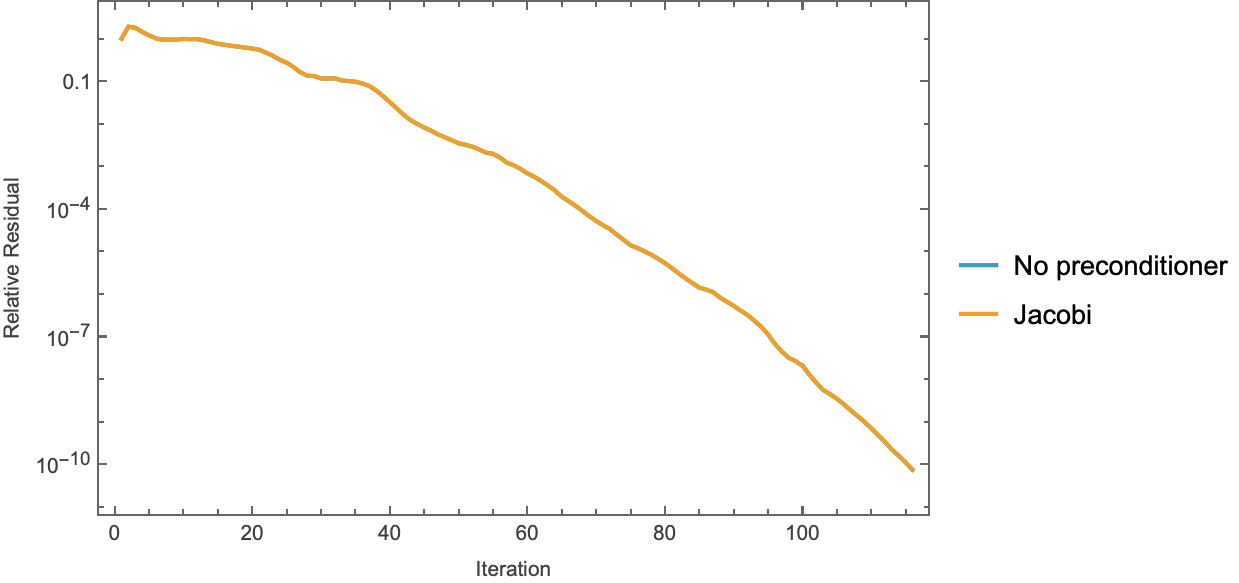
Both start the history at 1.0 (Sow[1.0] / res_hist = [1.0]), so iterations = len(res_hist) - 1 on both sides; both evaluate convergence on the post-step residual, so even the final iteration performs its (unused) preconditioner apply and direction update — the trajectories are state-identical, not merely output-identical. Two harmless implementation asymmetries: Mathematica’s initial state (line 72) calls precondFunc[vecB] twice where Python reuses z, and the default maxIter is 1000 vs Python’s 2000 — neither affects any converged run. The empirical check is necessarily qualitative, not bit-for-bit: the two languages draw the GRF noise from different generators (SeedRandom[42]/RandomVariate in Wolfram vs numpy’s PCG64 with seed 42), so the right-hand sides — and hence iteration counts — differ. Running wolframscript -file mathematica/poisson_pcg.wls prints 115 iterations at final relres $7.379\times 10^{-11}$ for both CG and Jacobi-PCG (figure ../figures/mma_convergence.png), versus Python’s 116 at $6.67\times 10^{-11}$ (results/baseline.json). What does transfer across languages is the structural signature: on each side CG and Jacobi-PCG are iteration-identical with matching residual histories (Mathematica reports $\Vert x_{\mathrm{none}} - x_{\mathrm{Jacobi}}\Vert = 2.0\times 10^{-16}$) — the scale-invariance proven in §4.1, reproduced independently by both implementations.
The convention M$\,\approx A^{-1}$ as an apply ($z = M(r)$, pcg.py line 37) is shared by every preconditioner in the repo: python/preconditioners.py (identity/Jacobi/ILU), python/nystrom.py, and the neural python/neural/npo.py.
4. Preconditioning: change of inner product, split-preconditioner equivalence
Let $M \approx A^{-1}$ be SPD (note: in this repo $M$ denotes the applied inverse, matching the code; textbooks often write $M \approx A$ and apply $M^{-1}$). Three equivalent constructions produce the algorithm of §3.1:
(a) Split preconditioner. Factor $M = E E^{\top}$ (e.g. Cholesky) and run plain CG on the SPD system
\[\hat{A}\, y = \hat{b}, \qquad \hat{A} = E^{\top} A E, \quad \hat{b} = E^{\top} b, \quad x = E y .\]Push the change of variables through the plain-CG recurrence: with $\hat{r}_k = E^{\top} r_k$, $\hat{p}_k = E^{-1} p_k$ one finds
$\hat{r}_k^{\top}\hat{r}_k = r_k^{\top} E E^{\top} r_k = r_k^{\top} M r_k = r_k^{\top} z_k$ and $\hat{p}_k^{\top}\hat{A}\hat{p}_k = p_k^{\top} A p_k$, so every scalar in the recurrence is computable from $A$, $M$-applies, and inner products — $E$ never appears. The result is exactly pcg with $z = M r$. Consequence: PCG’s convergence is governed by the spectrum of $\hat{A} = E^{\top} A E$, which is similar to $MA$; hence “the spectrum of the preconditioned operator $MA$” is the object of interest even though $MA$ is nonsymmetric.
(b) Change of inner product. $MA$ is self-adjoint and positive definite in the $M^{-1}$-inner product: $\langle MAu, v\rangle_{M^{-1}} = u^{\top} A v = \langle u, MAv\rangle_{M^{-1}}$. PCG is literally plain CG applied to $MAx = Mb$ with every Euclidean inner product replaced by $\langle\cdot,\cdot\rangle_{M^{-1}}$; the error functional being minimized is still $\Vert x - x^\star\Vert _A$, now over the preconditioned Krylov space $\mathcal{K}_k(MA,\, Mb)$.
(c) Polynomial view. $x_k = q_{k-1}(MA)\, Mb$: the preconditioner reshapes the spectrum that the optimal polynomial must be small on. Good preconditioning = clustering $\Lambda(MA)$, so a low-degree polynomial can nearly vanish on it.
4.1 Scale invariance of PCG in $M$ — why Jacobi $\equiv$ plain CG here
Theorem. Replacing $M$ by $cM$ for any constant $c > 0$ leaves every iterate $x_k$ and every residual $r_k$ of PCG unchanged.
Proof (induction on the state $(x, r, p, \rho)$). Under $M \to cM$: $z_k \to c z_k$, hence $\rho_k = r_k^{\top} z_k \to c\rho_k$ and initially $p_0 = z_0 \to c p_0$. Inductively assume $x_k, r_k$ unchanged and $p_k \to c p_k$, $\rho_k \to c\rho_k$. Then $\alpha_k = \rho_k/(p_k^{\top}Ap_k) \to c\rho_k/(c^2 p_k^{\top}Ap_k) = \alpha_k / c$, so $\alpha_k p_k$ is invariant: $x_{k+1}, r_{k+1}$ unchanged. Next $z_{k+1} \to c z_{k+1}$, $\rho_{k+1} \to c\rho_{k+1}$, $\beta_k = \rho_{k+1}/\rho_k$ invariant, and $p_{k+1} = z_{k+1} + \beta_k p_k \to c\, p_{k+1}$, closing the induction. $\square$
Now the punchline for the canonical problem: the constant-coefficient Dirichlet Laplacian has constant diagonal $\operatorname{diag}(A) = 4/h^2 = 4\cdot 33^2 = 4356$ (this is also the median eigenvalue: eig_A.median $= 4356.0$ in results/npo_spectrum.json). So the Jacobi preconditioner (preconditioners.py lines 22–41) is
a positive scalar multiple of the identity — by the theorem, Jacobi-PCG is iteration-identical to plain CG, differing only by float rounding. Measured (results/results.json, results/baseline.json):
| method | iterations | final relres |
|---|---|---|
| CG (none) | 116 | $6.666547523655469\times 10^{-11}$ |
| CG (Jacobi) | 116 | $6.666547523655465\times 10^{-11}$ |
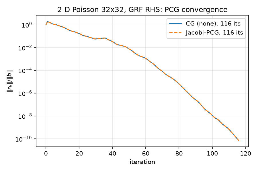
Maximum deviation between the two full residual histories: $4.441\times 10^{-16}$ — two ULPs. This is the sanity check jacobi_equals_none_constant_coeff: true asserted in python/experiments/run_all.py (lines 177–179, 254–261), visible as perfectly overlapping curves in ../figures/baseline_convergence.png.
The contrast case proves it’s the constancy of the diagonal, not weakness of Jacobi: on variable_poisson_2d(32, contrast=100) the diagonal jumps from $4/h^2 = 4356$ to $400/h^2 = 435600$ across the material interface (python/poisson.py lines 71–128), Jacobi is no longer $cI$, and it cuts iterations from 771 to 137 — a $5.6\times$ reduction (sanity check jacobi_beats_none_variable_coeff: true). Full discussion of Jacobi/ILU mechanics in 05-classical-preconditioners.md.
The same scale-invariance is load-bearing for the neural preconditioner: npo.py (module comment, lines 47–53) trains $M_\theta \approx \hat{A}^{-1}$ for the scaled operator $\hat{A} = h^2 A$ and uses it on $A$ unchanged, because $M_\theta \approx h^{-2}A^{-1}$ is a positive multiple of $A^{-1}$.
5. Convergence theory: the Chebyshev $\sqrt{\kappa}$ bound vs. reality
5.1 Derivation
From §1, $e_k = p_k(A)\,e_0$ with $p_k(0)=1$ chosen $A$-norm-optimally. Expanding $e_0$ in eigenvectors of $A$,
\[\Vert e_k\Vert _A \;=\; \min_{p_k(0)=1}\; \Vert p_k(A) e_0\Vert _A \;\le\; \min_{p_k(0)=1}\; \max_{\lambda \in \Lambda(A)} \vert p_k(\lambda)\vert \; \cdot \Vert e_0\Vert _A \;\le\; \min_{p_k(0)=1}\; \max_{\lambda \in [\lambda_{\min}, \lambda_{\max}]} \vert p_k(\lambda)\vert \;\cdot\Vert e_0\Vert _A .\]The last min–max problem is solved by shifted-and-scaled Chebyshev polynomials $p_k^\star(\lambda) = T_k!\big(\tfrac{\lambda_{\max}+\lambda_{\min}-2\lambda}{\lambda_{\max}-\lambda_{\min}}\big) \big/ T_k!\big(\tfrac{\lambda_{\max}+\lambda_{\min}}{\lambda_{\max}-\lambda_{\min}}\big)$, giving the classical bound
\[\frac{\Vert e_k\Vert _A}{\Vert e_0\Vert _A} \;\le\; \frac{2}{\rho^{-k} + \rho^{k}} \;\le\; 2\rho^{\,k}, \qquad \rho = \frac{\sqrt{\kappa}-1}{\sqrt{\kappa}+1}, \quad \kappa = \frac{\lambda_{\max}}{\lambda_{\min}} .\]Asymptotically $\rho \approx 1 - 2/\sqrt{\kappa}$, so $k \approx \tfrac{\sqrt{\kappa}}{2}\ln(2/\varepsilon)$ — the famous $O(\sqrt{\kappa})$ iteration complexity (vs. $O(\kappa)$ for steepest descent). Since the code stops on the 2-norm residual rather than the $A$-norm error, convert via $\Vert r_k\Vert 2 = \Vert e_k\Vert _{A^2} \le \sqrt{\lambda{\max}}\Vert e_k\Vert A$ and $\Vert e_0\Vert _A \le \Vert r_0\Vert _2/\sqrt{\lambda{\min}}$:
\[\frac{\Vert r_k\Vert _2}{\Vert b\Vert _2} \;\le\; 2\sqrt{\kappa}\;\rho^{\,k}.\]5.2 Predicted vs. measured
Plugging in the exact $\kappa(A) = 440.6886$ (results/spectra.json, kappa_analytic_exact $= 440.6885603836582$): $\sqrt{\kappa} = 20.993$, $\rho = 19.993/21.993 = 0.90906$, $\ln(1/\rho) = 0.09534$. For $\varepsilon = 10^{-10}$:
| bound | predicted $k$ | formula |
|---|---|---|
| $A$-norm error $\le \varepsilon$ | $\lceil \ln(2/\varepsilon)/\ln(1/\rho)\rceil = \mathbf{249}$ | $23.72/0.09534$ |
| relative residual $\le \varepsilon$ (as coded) | $\lceil \ln(2\sqrt{\kappa}/\varepsilon)/\ln(1/\rho)\rceil = \mathbf{281}$ | $26.76/0.09534$ |
| measured (results/results.json) | 116 (final relres $6.67\times 10^{-11}$) |
The bound is pessimistic by a factor of $\sim 2.1$–$2.4$ ($249/116 = 2.15$, $281/116 = 2.42$). Equivalently: the observed geometric-mean convergence factor is $(6.67\times 10^{-11})^{1/116} = 0.817$ per iteration versus the bound’s $\rho = 0.909$. Three compounding reasons:
- The bound only sees the endpoints $[\lambda_{\min}, \lambda_{\max}]$. The true minimization is over the 1024 discrete eigenvalues (at most 528 distinct, §1). The optimal polynomial exploits gaps: once low-degree factors have effectively annihilated the outermost eigenvalues, the remaining convergence is governed by an effective condition number of the interior spectrum — the mechanism behind CG’s well-known superlinear convergence.
- Eigenvalue multiplicity and clustering. The 2-D Laplacian spectrum $(\lambda^{(1)}_k+\lambda^{(1)}_l)/h^2$ is dense in the middle (82.0% of eigenvalues lie within $[0.5, 2]\times$ the median 4356 —
eig_A.frac_within_half_to_2x_medianin results/npo_spectrum.json): a polynomial that is small on that bulk plus a handful of stragglers needs far fewer degrees than the interval bound assumes. - The RHS is not adversarial. The Chebyshev bound is worst-case over $e_0$. Our $b$ is a GRF with spectral density $(\vert k\vert ^2+\tau^2)^{-1}$ (03-gaussian-random-fields.md): its components along the rough, high-$\lambda$ eigenvectors are strongly damped, so the error CG must remove barely excites the top of the spectrum.
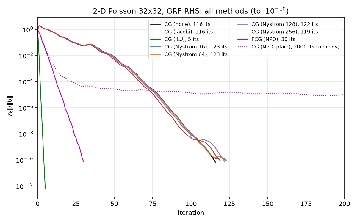
Two instructive extremes from the same benchmark (results/results.json, figure ../figures/all_convergence.png):
- ILU: 5 iterations to relres $6.21\times 10^{-13}$ — the preconditioned spectrum is so tightly clustered near 1 that a degree-5 polynomial suffices; endpoint-based $\kappa$ reasoning is irrelevant. See 05-classical-preconditioners.md.
- Nyström rank 16: exact preconditioned $\kappa = 439.62 < 440.69$ (results/nystrom.json) yet 123 iterations $> 116$. A (marginally) smaller $\kappa$ does not guarantee fewer iterations — the randomized sketch slightly rearranges the interior spectrum, and on this flat-top Laplacian spectrum that distortion outweighs the negligible endpoint gain. Iteration counts by rank: 123, 123, 122, 119 for ranks 16, 64, 128, 256 (
nystrom_iterations_by_rank; note the reported-not-asserted tie 123==123 in the strict-monotonicity sanity check, run_all.py lines 183–189). Full analysis in 07-nystrom-preconditioning.md.
The moral, which recurs in §6: clustering of $\Lambda(MA)$ is the real predictor; $\kappa$ is only a proxy.
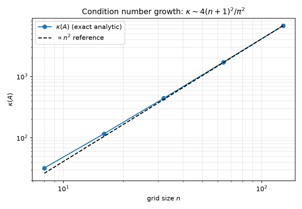
For scaling in $n$: $\kappa \sim 4(n+1)^2/\pi^2$, so CG iterations grow like $O(n) = O(\sqrt{\kappa})$; $\kappa$ values 32.16, 116.46, 440.69, 1711.66, 6743.68 for $n = 8, 16, 32, 64, 128$ with $\kappa/n^2 \to \approx 0.41$ (results/spectra.json, figure ../figures/kappa_scaling.png; derivation in 02-eigenvalues.md).
6. Flexible CG: Polak–Ribière $\beta$ and nonlinear preconditioners
6.1 The derivation that makes PR inevitable
Suppose the preconditioner changes from iteration to iteration — $z_k = M_k(r_k)$ with $M_k$ possibly nonlinear, as with the NPO where the ReLU network is not any fixed matrix. The global orthogonality structure of §2 is gone; the best we can do is enforce local $A$-conjugacy $p_{k+1}^{\top} A p_k = 0$ exactly, by construction. With $p_{k+1} = z_{k+1} + \beta_k p_k$:
\[\beta_k \;=\; -\frac{z_{k+1}^{\top} A p_k}{p_k^{\top} A p_k} \;\overset{A p_k = (r_k - r_{k+1})/\alpha_k}{=}\; \frac{z_{k+1}^{\top}(r_{k+1} - r_k)}{\alpha_k\, p_k^{\top} A p_k} \;=\; \boxed{\ \frac{z_{k+1}^{\top}(r_{k+1} - r_k)}{z_k^{\top} r_k}\ }\]using $\alpha_k p_k^{\top} A p_k = r_k^{\top} z_k$ from the line-search formula. This is the Polak–Ribière $\beta$ of Notay, Flexible Conjugate Gradients, SIAM J. Sci. Comput. 22(4), 2000: it makes consecutive directions exactly $A$-conjugate for any preconditioner whatsoever, because the only identity it uses is the residual update itself.
The Fletcher–Reeves form $\beta_k^{FR} = \frac{r_{k+1}^{\top} z_{k+1}}{r_k^{\top} z_k}$ used by classical PCG differs from PR by the term $\frac{z_{k+1}^{\top} r_k}{z_k^{\top} r_k}$. For a fixed SPD $M$ that term vanishes: $z_{k+1}^{\top} r_k = r_{k+1}^{\top} M r_k = r_{k+1}^{\top} z_k = 0$ by symmetry of $M$ plus the exact-PCG orthogonality $r_{k+1} \perp_{\,} z_k$. For a nonlinear, nonsymmetric $M_\theta$ neither ingredient holds, so FR’s $\beta$ carries a spurious component, $p_{k+1}$ loses $A$-conjugacy even with its immediate predecessor, and the “line searches” start fighting each other — the method degrades toward (erratic) preconditioned steepest descent and stalls once the accumulated non-conjugacy balances the per-step reduction.
6.2 The implementation delta
python/pcg.py flexible_pcg (lines 126–139) is identical to pcg except:
beta = (z_new @ (r_new - r)) / rz   # line 134: Polak-Ribiere (Notay 2000)
p = z_new + beta * p
with rz holding the previous $z_k^{\top} r_k$. Cost: the same one matvec + one $M$-apply per iteration, plus one extra stored vector (the previous residual r, needed for $r_{k+1}-r_k$), one extra AXPY-sized subtraction, and one extra inner product — pcg computes two per iteration ($p^{\top}Ap$, $r^{\top}z$) where flexible_pcg computes three ($p^{\top}Ap$, $z_{k+1}^{\top}(r_{k+1}-r_k)$, $r^{\top}z$; lines 128, 134, 137). All $O(N)$ and negligible next to the matvec.
6.3 Measured: NPO with plain vs. flexible PCG
The trained NPO (06-neural-preconditioner.md, NPO paper: Li, Xiao, Lai & Wang, Neural Preconditioning Operator for Efficient PDE Solves, https://arxiv.org/abs/2502.01337) is quantifiably far from a fixed SPD matrix (results/npo_spectrum.json, computed by python/experiments/npo_spectrum.py):
- nonsymmetry of the column linearization $\tilde{M}$ (with $\tilde{M}{:,j} = M\theta(e_j)$): $\Vert \tilde{M}-\tilde{M}^{\top}\Vert _F/\Vert \tilde{M}\Vert _F = 0.568$;
- nonlinearity: $\Vert \tilde{M} b - M_\theta(b)\Vert / \Vert M_\theta(b)\Vert = 0.432$ on the canonical GRF $b$ — the linearization mispredicts the actual apply by 43%. (The wrapper is positively homogeneous, $M_\theta(cr) = c\,M_\theta(r)$ for $c>0$, by unit-norm input normalization — npo.py lines 218–227 — but homogeneity is much weaker than linearity.)
Results on the canonical problem (results/results.json, reproduced in results/npo_eval.json; figure ../figures/npo_convergence.png):
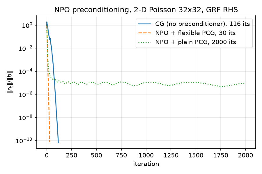
| solver | iterations | final relres | converged |
|---|---|---|---|
| CG, no preconditioner | 116 | $6.67\times 10^{-11}$ | yes |
| FCG (NPO, Notay PR $\beta$) | 30 | $7.16\times 10^{-11}$ | yes |
| CG (NPO, plain FR $\beta$) | 2000 (max) | $9.65\times 10^{-6}$ | no — stalls near $10^{-5}$ |
The plain-PCG run is a deliberate negative control (python/neural/eval_npo.py lines 9–11, 50): identical preconditioner, identical everything, only $\beta^{FR}$ vs $\beta^{PR}$ — and it stalls five orders of magnitude short after $67\times$ more iterations (1.68 s vs 0.028 s solve wall time). Flexible CG converges in 30 iterations, a $116/30 = 3.87\times$ reduction over plain CG (speedup_fcg_vs_cg $= 3.8667$).
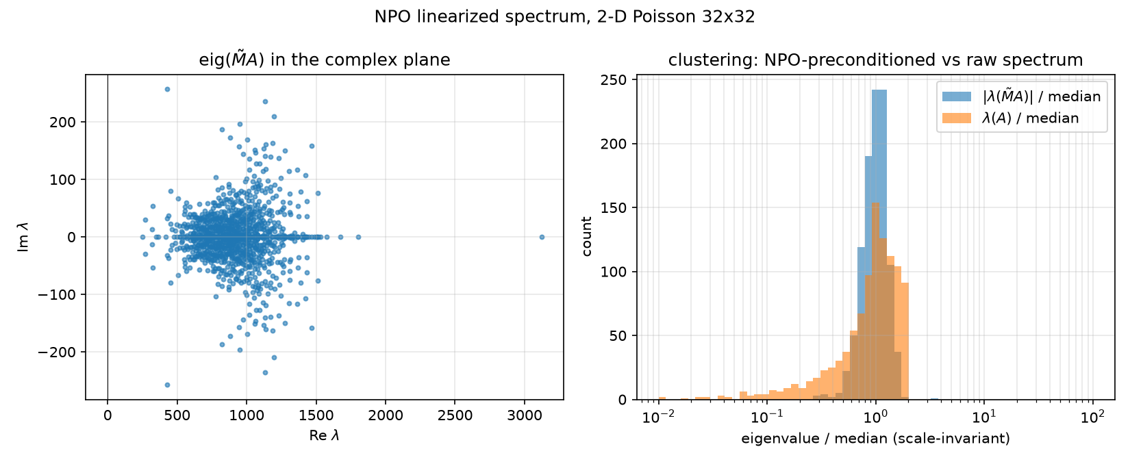
Why 30 works: clustering, not symmetry. The linearized preconditioned spectrum $\operatorname{eig}(\tilde{M}A)$ has all 1024 eigenvalues in the open right half-plane ($\mathrm{Re}\,\lambda \in [248.8,\ 3125.2]$, $\max\vert \mathrm{Im}\,\lambda\vert = 257.1$, zero nonpositive real parts) with spread $\max\vert \lambda\vert /\min\vert \lambda\vert = 12.56$ versus $\kappa(A) = 440.69$ — $35\times$ tighter — and 98.1% of eigenvalues within $[0.5, 2]\times$ the median versus 82.0% for $A$ (figure ../figures/npo_spectrum.png). Feeding the spread into the Chebyshev heuristic as if it were a condition number: $\sqrt{12.56} = 3.54$, $\rho_{\mathrm{eff}} = 0.560$, predicted $k \approx \ln(2\cdot 10^{10})/\ln(1/0.560) \approx 41$ — the actual 30 (observed factor $0.459$/iteration) again beats the endpoint bound, for the same clustering reasons as §5.2. None of the classical theory applies rigorously here (the operator isn’t even linear), but the scale-invariant clustering diagnostic predicts the behavior well — which is exactly why npo_spectrum.py measures median-relative clustering rather than a raw “$\kappa$”.
7. GMRES vs. CG (and where FCG sits)
The NPO paper (https://arxiv.org/abs/2502.01337) deploys its preconditioner inside GMRES; this repo uses flexible CG. Both are Krylov methods — iterates from $\mathcal{K}_k(MA, Mb)$ — differing in which optimality they enforce and what that costs:
| CG | flexible CG (Notay) | GMRES / FGMRES | |
|---|---|---|---|
| optimality | global $\min \Vert e_k\Vert _A$ over $\mathcal{K}_k$ | local only ($p_{k+1} \perp_A p_k$); global optimality not guaranteed | global $\min \Vert r_k\Vert _2$ over $\mathcal{K}_k$ |
| requires | $A$ SPD, fixed SPD $M$ | $A$ SPD; $M$ arbitrary (varying/nonlinear) | any nonsingular $A$; FGMRES allows varying $M$ |
| recurrence | 2-term coupled; $O(1)$ vectors | 2-term + 1 extra vector | full Arnoldi orthogonalization: $k$ vectors, $O(Nk)$ work at step $k$ (or restarts, losing optimality) |
| per-iteration cost here | 1 matvec + 1 $M$-apply + $O(N)$ | same + $O(N)$ | 1 matvec + 1 $M$-apply + $O(Nk)$ |
GMRES is the conservative choice when the preconditioned operator may be badly nonsymmetric or indefinite — its residual is monotone by construction, and FGMRES (Saad 1993) tolerates a different $M_k$ each step by storing both Arnoldi bases. The NPO paper needs that generality across its PDE suite. Here, the measured linearized spectrum of $\tilde{M}A$ is entirely in the right half-plane with small imaginary parts and heavy clustering (§6.3), and $A$ itself is SPD — precisely the regime where Notay showed local $A$-conjugacy is enough in practice. FCG then delivers Krylov acceleration at CG-like memory ($O(1)$ vectors vs GMRES’s $O(k)$: at $k=30$ that is ~30 stored basis vectors of length 1024 plus a growing Hessenberg least-squares problem, vs. 5–6 vectors total for FCG). The empirical justification is the table in §6.3: FCG converges in 30 iterations to $7.2\times 10^{-11}$ with true-residual accuracy confirmed against a direct solve (relerr_vs_spsolve $= 3.10\times 10^{-11}$).
Summary of load-bearing facts (all from results/ JSONs)
- CG = $A$-norm-optimal polynomial method on $\mathcal{K}_k(A,b)$; the 5-line loop in pcg.py (lines 67–79) is state-identical to Mathematica
pcgStep(poisson_pcg.wls lines 59–68), Saad Alg. 9.1. - Chebyshev bound with exact $\kappa = 440.6886$ predicts 249 ($A$-norm) / 281 (residual) iterations at $10^{-10}$; measured: 116 — pessimistic $\sim 2.1$–$2.4\times$ because the bound ignores spectral clustering (82% of $\Lambda(A)$ within $[0.5,2]\times$ median) and RHS smoothness.
- PCG is invariant under $M \to cM$, $c>0$; since $\operatorname{diag}(A) \equiv 4/h^2 = 4356$, Jacobi $= \frac{h^2}{4}I$ and matches plain CG to $4.4\times 10^{-16}$ over the whole residual history (116 = 116 its). On the variable-coefficient problem (diagonal 4356 → 435600) Jacobi wins 137 vs 771. See 05-classical-preconditioners.md.
- Smaller exact $\kappa$ does not imply fewer iterations: Nyström rank 16 has $\kappa_{\mathrm{prec}} = 439.62 < 440.69$ but takes 123 > 116 iterations. See 07-nystrom-preconditioning.md.
- Polak–Ribière $\beta = z_{k+1}^{\top}(r_{k+1}-r_k)/z_k^{\top}r_k$ enforces exact local $A$-conjugacy for any preconditioner; Fletcher–Reeves equals it only for fixed SPD $M$. With the nonlinear NPO (nonsymmetry 0.568, nonlinearity 0.432), FR-PCG stalls at $9.65\times 10^{-6}$ after 2000 iterations while PR-FCG converges in 30 ($3.87\times$ fewer than plain CG), driven by a $35\times$ tighter, 98.1%-clustered right-half-plane spectrum of $\tilde{M}A$. See 06-neural-preconditioner.md.
- GMRES (used by the NPO paper) and (F)CG optimize $\Vert r\Vert _2$ vs $\Vert e\Vert _A$ over the same Krylov spaces; FCG trades guaranteed global optimality for $O(1)$ memory, and the measured spectrum justifies that trade here.
Full cross-method numbers and figures: 08-results.md.