Learning Rotations Online: Two Pairs at a Time
The batch-size-2 mirror of Learning Rotations Online: same unknown rotation, same three update philosophies — but each step now delivers two observations at once.
An unknown rotation \(A \in SO(d)\) is observed through pairs \((x, y = Ax)\), with \(x\) uniform on the unit sphere. The estimate \(W\) starts at \(I\); in this variant every step delivers two independent pairs, stacked as columns \(X = [\,x_1\; x_2\,]\), \(Y = [\,y_1\; y_2\,]\). As before, the amount of rotation structure the update exploits sets the convergence rate — and batching turns out to be exactly free.
Three ways to insert two facts
1 · Gradient descent — few assumptions
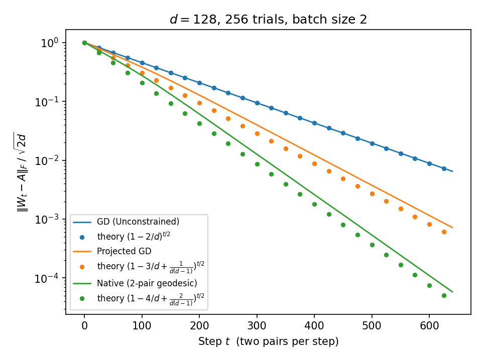
The smallest change to \(W\) that fits both pairs at once — a block Kaczmarz step (for one pair it reduces to the rank-one update \(W + (y - Wx)x^\top\)). It works for any matrix; \(W\) drifts off \(SO(d)\). The error obeys the exact identity \(W' - A = (W - A)(I - P)\), with \(P\) now the projector onto the random plane \(\mathrm{span}\{x_1, x_2\}\): each step wipes the error out of two random directions instead of one.
squared error × \(1 - 2/d\) per step, exact2 · Gradient descent + projection
The same step, snapped back to the nearest rotation. In the misalignment variable the pre-projection matrix is \(I + \Omega(I - P)\) exactly, and the polar factor keeps its skew part: \(\Omega \mapsto \Omega - (P\Omega + \Omega P)/2\) — the same half-correction as at batch one, with a rank-2 \(P\).
squared error × \(1 - 3/d + \frac{1}{d(d-1)}\) per step3 · A native update for rotations
Rotate \(W\) by the smallest rotation that fixes both predictions exactly. This is precisely the trace-maximal orthogonal completion of the two constraints: it lives in the \(\le 4\)-dimensional subspace \(\mathrm{span}\{Wx_1, Wx_2, y_1, y_2\}\), and the single-pair Rodrigues rotation \(I + K + K^2/(1+c)\) is its one-constraint special case. It even has an SVD-free closed form in the same spirit — two Rodrigues rotations and one arctangent: see the two-batch Rodrigues formula below.
squared error × \(1 - 4/d + \frac{2}{d(d-1)}\) per stepResult
| Update | Uses | Contraction of \(\mathbb{E}\Vert W - A \Vert_F^2\) |
|---|---|---|
| Gradient descent | nothing | \(1 - 2/d\), exact |
| GD + projection | additive update, project to SO | \(1 - 3/d + \tfrac{1}{d(d-1)}\) |
| Native | multiplicative update, maintaining SO | \(1 - 4/d + \tfrac{2}{d(d-1)}\) |
To leading order the constants are 2 : 3 : 4 — the batch-1 constants, doubled.
The ratio 1 : 1.5 : 2 is invariant under batching.
Is batching worth it?
Per sample, nothing changes to leading order: two pairs at a time contracts squared error by \(1 - 2b/d + \cdots\) per step for the native update, which is \((1 - 2/d)\)-per-sample twice over. The curves below overlap so closely that the dashed batch-1 runs hide behind the solid batch-2 ones.
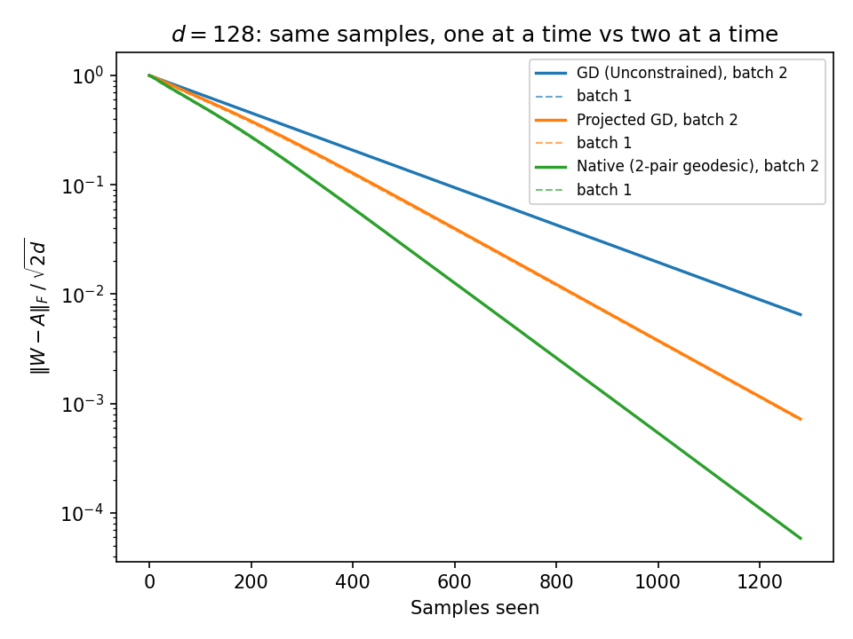
At second order, batching is strictly better — for gradient descent,
$$1 - \frac{2}{d} \;<\; \left(1 - \frac{1}{d}\right)^2 = 1 - \frac{2}{d} + \frac{1}{d^2},$$and for the native update \(1 - 4/d + \tfrac{2}{d(d-1)} < (1 - 2/d)^2 = 1 - 4/d + \tfrac{4}{d^2}\) for every \(d > 2\). Two sequential steps waste the overlap between their random directions; the batch step never re-corrects what it already fixed. The advantage is \(O(1/d^2)\) per step — real, but invisible at \(d = 128\).
The two-batch Rodrigues formula
The argmin in update 3 needs no SVD. Like the single-pair Rodrigues rotation, it can be assembled from inner products alone: two plane rotations satisfy the constraints, and one arctangent makes the result the smallest such rotation. Write \(u_1 = Wx_1\), \(u_2 = Wx_2\); all four of \(u_1, u_2, y_1, y_2\) are unit vectors, and \(u_1 \cdot u_2 = y_1 \cdot y_2 = x_1 \cdot x_2\) automatically.
Step 1 — align the first pair. A single-pair Rodrigues rotation, applied also to \(u_2\):
$$R_1 = I + K_1 + \frac{K_1^2}{1 + u_1 \cdot y_1}, \qquad K_1 = y_1 u_1^\top - u_1 y_1^\top, \qquad u_2 \leftarrow R_1 u_2 .$$Step 2 — align the second pair without disturbing the first. Split off the \(y_1\)-components: with \(a = y_1 \cdot y_2\) (which automatically equals \(y_1 \cdot u_2\) after step 1),
$$p = u_2 - a\,y_1, \qquad q = y_2 - a\,y_1, \qquad \lVert p \rVert = \lVert q \rVert = \sqrt{1 - a^2},$$and rotate \(\hat p\) onto \(\hat q\) with a second Rodrigues rotation, \(R_2 = I + K_2 + K_2^2/(1 + \hat p \cdot \hat q)\), \(K_2 = \hat q \hat p^\top - \hat p \hat q^\top\). Its plane is orthogonal to \(y_1\), so the first constraint survives: \(R_2 R_1\) now satisfies both.
Step 3 — spend the leftover freedom on the trace. \(R_2 R_1\) is feasible but not yet minimal. The smallest feasible rotation acts only on the active 4-space \(\mathrm{span}\{u_1, u_2, y_1, y_2\}\) — turning anything outside it costs trace and satisfies no constraint, the same localization as in the trace-maximal completion — and every feasible rotation acting only there is \(R_2 R_1 Q\), where \(Q\) turns the one plane inside it that the constraints cannot see: \(Z\), the orthogonal complement of \(\mathrm{span}\{u_1, u_2\}\) within the 4-space. Build an orthonormal basis \(z_1, z_2\) of \(Z\) (Gram–Schmidt of \(y_1, y_2\) against the orthonormalized \(u\)'s) and set
$$\alpha = z_1 \cdot R_2 R_1 z_1 + z_2 \cdot R_2 R_1 z_2, \qquad \beta = z_1 \cdot R_2 R_1 z_2 - z_2 \cdot R_2 R_1 z_1, \qquad \theta^\star = \mathrm{atan2}(\beta, \alpha),$$and let \(Q\) rotate \(Z\) by \(\theta^\star\) — the same two-coefficient trace maximization that produced the half-angle in the projected-GD analysis, and that picks the proper-rotation optimum directly (no determinant correction needed).
The update is \(W \leftarrow R_2 R_1 Q\, W\): three plane rotations, each applied as a rank-2 correction. Forming the factors costs a handful of inner products and one atan2 — \(O(d)\); only applying them to \(W\) is \(O(d^2)\), and nothing larger than a scalar trigonometric pair is ever solved for. Implemented as native_step_rodrigues2 alongside the subspace-SVD route, the two agree to \(10^{-14}\) across random instances, near convergence, and from cold start — the simulation script asserts this on every run. That agreement also confirms the circle parametrization within the active subspace: the SVD route searches the full completion freedom there, so any angle the circle missed would show up as a trace gap. (Probability-zero antipodal alignments fall back to the SVD route.) Steps 1–2 alone already satisfy the constraints and match the optimum to first order near convergence; step 3 is what makes the update exactly the smallest feasible rotation at any distance.
Where the constants come from
Write \(W = (I + \Omega)A\) with \(\Omega\) small and skew, and let \(P\) project onto \(\mathrm{span}\{y_1, y_2\}\). The three updates linearize exactly as at batch one, with rank-2 \(P\):
$$\text{GD:}\;\; \Omega \mapsto \Omega(I - P) \qquad \text{PGD:}\;\; \Omega \mapsto \Omega - \tfrac{1}{2}(P\Omega + \Omega P) \qquad \text{Native:}\;\; \Omega \mapsto (I - P)\,\Omega\,(I - P)$$Two expectation facts close the computation. First, \(\mathbb{E}[P] = (2/d)I\). Second — the genuinely new ingredient at batch \(\ge 2\) —
$$\mathbb{E}\,\lVert P \Omega P \rVert_F^2 \;=\; \frac{2\,\lVert \Omega \rVert_F^2}{d(d-1)},$$the expected size of the error's in-batch skew component, the part of \(\Omega\) that lives inside the random plane itself. At batch one this term is identically zero (\(y^\top \Omega y = 0\) for skew \(\Omega\)); at batch two it is what separates the exact constants \(3 - \tfrac{1}{d-1}\) and \(4 - \tfrac{2}{d-1}\) from the round numbers 3 and 4. Expanding the squared norms of the three maps and taking expectations gives the table above.
The same computation runs verbatim for batch size \(b\) (with \(\mathbb{E}[P] = (b/d)I\) and \(\mathbb{E}\Vert P\Omega P\Vert_F^2 = \tfrac{b(b-1)}{d(d-1)}\Vert\Omega\Vert_F^2\)):
$$\text{GD: } 1 - \frac{b}{d} \qquad \text{PGD: } 1 - \frac{3b}{2d} + \frac{b(b-1)}{2d(d-1)} \qquad \text{Native: } 1 - \frac{2b}{d} + \frac{b(b-1)}{d(d-1)}.$$As a sanity check, at \(b = d\) all three contractions hit exactly zero: a full batch determines \(W\), and every method converges in one step. The formulas know.
Implementation
The simulation is batch_two_collapse.py: the block-Kaczmarz step is a closed-form \(2\times 2\) solve, the native update is implemented twice — the subspace route (batched \(4 \times 4\) SVDs) and the two-batch Rodrigues closed form above, agreeing to \(10^{-14}\) — and only the projected-GD baseline pays for a dense polar decomposition. One honest engineering note: in batched NumPy the Rodrigues form is not the faster of the two (it makes a few dozen memory-bound passes over the trial stack where the subspace route fuses its work into a few GEMMs); its advantages are the explicit formula and the \(O(d)\) cost of forming the rotation, which is what matters when updates are applied one at a time. Orthogonality drift after 640 steps: \(8 \times 10^{-15}\); final constraint residual: \(2 \times 10^{-15}\).
python batch_two_collapse.py # simulate, fit constants, regenerate both figures